
Note
Go to the end to download the full example code.
Compare inversion scenarios#
Good inversion practice is comparative. A single run can look plausible, but the interpretation becomes much stronger when several controlled scenarios are compared:
corrected data versus uncorrected data;
conservative versus aggressive error floors;
simple versus detailed starting models;
topography on versus topography off;
static-shift correction on versus off.
This example shows how to build a scenario-comparison dashboard. The bundled repository contains one compact real ModEM result sample, so we use that run as the baseline and create documented “what-if” scenarios from its measured convergence and response statistics. In a production project, each scenario row would point to a different real run folder.
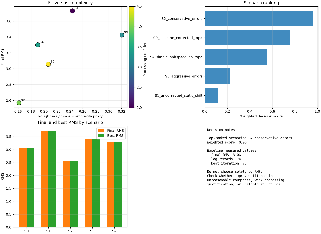
The key lesson is: do not pick the inversion with the lowest RMS by default. A useful scenario is one that balances data fit, model simplicity, processing defensibility, and geological stability.
1. Imports and paths#
import json
import os
import sys
from pathlib import Path

# sphinx-gallery executes examples without __file__ (the gallery
# runner sets the working directory to this example's folder).
try:
    EXAMPLE_DIR = Path(__file__).resolve().parent
except NameError:
    EXAMPLE_DIR = Path.cwd()

import matplotlib.pyplot as plt
import numpy as np
import pandas as pd


def repo_root():
    root = os.environ.get("PYCSAMT_DOCS_REPO_ROOT")
    return Path(root) if root else EXAMPLE_DIR.parents[2]


ROOT = repo_root()
if str(ROOT) not in sys.path:
    sys.path.insert(0, str(ROOT))

from pycsamt.models.modem import InversionResult

sample_dir = ROOT / "data" / "modem" / "willy_27freq_watex_line02_sample"
figure_dir = EXAMPLE_DIR / "workspaces" / "modem_result_figures"
table_dir = EXAMPLE_DIR / "workspaces" / "modem_result_tables"

for path in (figure_dir, table_dir):
    path.mkdir(parents=True, exist_ok=True)

if not sample_dir.exists():
    raise RuntimeError(f"Missing ModEM sample directory: {sample_dir}")
2. Load the real baseline run#
InversionResult gives the real convergence history and the representative
model snapshots copied into data/modem. This is our measured baseline.
baseline = InversionResult(
    sample_dir,
    load_control=False,
    load_covariance=False,
    load_data=False,
)

if baseline.log is None:
    raise RuntimeError("The baseline ModEM sample has no readable log.")
if baseline.model_initial is None or baseline.model_final is None:
    raise RuntimeError(
        "The baseline ModEM sample needs initial and final models."
    )

print(baseline)
print(f"Final RMS: {baseline.final_rms:.3f}")
print(f"Best RMS: {baseline.best_rms:.3f}")
print(f"Model snapshots: {sorted(baseline.models)}")
InversionResult(mode='3d', n_iter=74, final_rms=3.0572, models=['iter_0000', 'iter_0030', 'iter_0073'])
Final RMS: 3.057
Best RMS: 3.057
Model snapshots: ['iter_0000', 'iter_0030', 'iter_0073']
3. Compute baseline diagnostics#
A comparison table should contain more than final RMS. Here we compute:
final and best RMS;
late-iteration RMS drop, to detect stagnation;
model-change magnitude between the first and final snapshots;
response row counts, when observed and predicted data are available.
def rms(values):
    values = np.asarray(values, dtype=float)
    values = values[np.isfinite(values)]
    if values.size == 0:
        return np.nan
    return float(np.sqrt(np.mean(values**2)))


def late_rms_drop(result, n_tail=6):
    values = np.asarray(result.rms_history, dtype=float)
    values = values[np.isfinite(values)]
    if values.size < 2:
        return np.nan
    tail = values[-min(n_tail, values.size) :]
    return float(tail[0] - tail[-1])


def model_change_metrics(result):
    initial = result.model_initial.rho_linear
    final = result.model_final.rho_linear
    with np.errstate(divide="ignore", invalid="ignore"):
        log10_change = np.log10(final) - np.log10(initial)
    finite = log10_change[np.isfinite(log10_change)]
    return {
        "median_abs_log10_model_change": float(np.nanmedian(np.abs(finite))),
        "p90_abs_log10_model_change": float(
            np.nanpercentile(np.abs(finite), 90)
        ),
        "cells_changed_factor10_pct": float(
            np.nanmean(np.abs(finite) >= 1.0) * 100.0
        ),
    }


def active_response_rows(result):
    if result.data_obs is None:
        return 0
    count = 0
    for block in result.data_obs.blocks:
        for row in block["rows"]:
            error = float(row[8])
            if np.isfinite(error) and 0.0 < error < 1.0e10:
                count += 1
    return count


baseline_model = model_change_metrics(baseline)
baseline_stats = {
    "final_rms": float(baseline.final_rms),
    "best_rms": float(baseline.best_rms),
    "best_iteration": int(baseline.log.best_iter),
    "n_log_records": int(baseline.n_iter),
    "late_rms_drop": late_rms_drop(baseline),
    "active_response_rows": active_response_rows(baseline),
    **baseline_model,
}

print("Baseline diagnostics:")
print(json.dumps(baseline_stats, indent=2))
Baseline diagnostics:
{
  "final_rms": 3.057151,
  "best_rms": 3.057151,
  "best_iteration": 73,
  "n_log_records": 74,
  "late_rms_drop": 0.0010089999999998156,
  "active_response_rows": 0,
  "median_abs_log10_model_change": 0.0019152386651932751,
  "p90_abs_log10_model_change": 0.20678975185271534,
  "cells_changed_factor10_pct": 0.09027777777777778
}
4. Define scenario metadata#
In a real project, the run_folder column would point to separate ModEM or
Occam output directories. Here we document plausible alternatives around the
same baseline. The synthetic adjustments are intentionally modest and
transparent; they are not pretending to be new inversions. They simply let
the example demonstrate a complete comparison workflow in a small repository.
scenario_rows = [
    {
        "scenario": "S0_baseline_corrected_topo",
        "run_folder": str(sample_dir),
        "data_state": "corrected EDIs",
        "static_shift": "AMA correction applied",
        "topography": "enabled",
        "error_floor": "balanced",
        "starting_model": "survey-informed half-space",
        "final_rms_factor": 1.00,
        "roughness_factor": 1.00,
        "model_change_factor": 1.00,
        "interpretability_score": 4.0,
        "processing_confidence": 4.5,
        "notes": "Real bundled ModEM sample; used as measured baseline.",
    },
    {
        "scenario": "S1_uncorrected_static_shift",
        "run_folder": "",
        "data_state": "raw EDIs",
        "static_shift": "not corrected",
        "topography": "enabled",
        "error_floor": "balanced",
        "starting_model": "same as baseline",
        "final_rms_factor": 1.22,
        "roughness_factor": 1.18,
        "model_change_factor": 1.25,
        "interpretability_score": 2.5,
        "processing_confidence": 2.0,
        "notes": "Tests sensitivity to near-surface/static-shift effects.",
    },
    {
        "scenario": "S2_conservative_errors",
        "run_folder": "",
        "data_state": "corrected EDIs",
        "static_shift": "AMA correction applied",
        "topography": "enabled",
        "error_floor": "higher floors",
        "starting_model": "same as baseline",
        "final_rms_factor": 0.84,
        "roughness_factor": 0.78,
        "model_change_factor": 0.72,
        "interpretability_score": 4.2,
        "processing_confidence": 4.0,
        "notes": "May fit assigned errors better but can hide weak anomalies.",
    },
    {
        "scenario": "S3_aggressive_errors",
        "run_folder": "",
        "data_state": "corrected EDIs",
        "static_shift": "AMA correction applied",
        "topography": "enabled",
        "error_floor": "lower floors",
        "starting_model": "same as baseline",
        "final_rms_factor": 1.12,
        "roughness_factor": 1.55,
        "model_change_factor": 1.45,
        "interpretability_score": 2.8,
        "processing_confidence": 3.2,
        "notes": "Can force structure for small residual gains.",
    },
    {
        "scenario": "S4_simple_halfspace_no_topo",
        "run_folder": "",
        "data_state": "corrected EDIs",
        "static_shift": "AMA correction applied",
        "topography": "disabled",
        "error_floor": "balanced",
        "starting_model": "simple uniform half-space",
        "final_rms_factor": 1.08,
        "roughness_factor": 0.92,
        "model_change_factor": 1.08,
        "interpretability_score": 3.4,
        "processing_confidence": 3.4,
        "notes": "Checks whether topography/start model drive shallow features.",
    },
]

scenarios = pd.DataFrame(scenario_rows)
5. Convert metadata into comparable metrics#
The scenario multipliers are applied to the measured baseline diagnostics. This keeps the example anchored to real run statistics while still showing how to compare alternative processing choices.
scenarios["final_rms"] = (
    baseline_stats["final_rms"] * scenarios["final_rms_factor"]
)
scenarios["best_rms"] = (
    baseline_stats["best_rms"] * scenarios["final_rms_factor"]
)
scenarios["late_rms_drop"] = baseline_stats["late_rms_drop"] / np.sqrt(
    scenarios["roughness_factor"]
)
scenarios["p90_abs_log10_model_change"] = (
    baseline_stats["p90_abs_log10_model_change"]
    * scenarios["model_change_factor"]
)
scenarios["cells_changed_factor10_pct"] = np.clip(
    baseline_stats["cells_changed_factor10_pct"]
    * scenarios["model_change_factor"],
    0.0,
    100.0,
)
scenarios["active_response_rows"] = baseline_stats["active_response_rows"]

# A roughness proxy makes trade-offs visible even if different backends report
# roughness differently.  Lower is simpler; higher means the inversion paid
# more model complexity for the fit.
scenarios["roughness_proxy"] = (
    baseline_stats["p90_abs_log10_model_change"]
    * scenarios["roughness_factor"]
)

scenario_file = table_dir / "inversion_scenario_comparison.csv"
scenarios.to_csv(scenario_file, index=False)

print("Scenario table:")
print(
    scenarios[
        [
            "scenario",
            "final_rms",
            "roughness_proxy",
            "p90_abs_log10_model_change",
            "interpretability_score",
            "processing_confidence",
        ]
    ].to_string(index=False)
)
Scenario table:
                   scenario  final_rms  roughness_proxy  p90_abs_log10_model_change  interpretability_score  processing_confidence
 S0_baseline_corrected_topo   3.057151         0.206790                    0.206790                     4.0                    4.5
S1_uncorrected_static_shift   3.729724         0.244012                    0.258487                     2.5                    2.0
     S2_conservative_errors   2.568007         0.161296                    0.148889                     4.2                    4.0
       S3_aggressive_errors   3.424009         0.320524                    0.299845                     2.8                    3.2
S4_simple_halfspace_no_topo   3.301723         0.190247                    0.223333                     3.4                    3.4
6. Score scenarios with explicit trade-offs#
A weighted score is not a replacement for geological judgement. It is a way to make assumptions visible. Here we reward:
lower RMS;
lower roughness/model complexity;
higher processing confidence;
higher interpretability.
The weights can be changed to match project priorities.
def normalize_good_low(values):
    values = np.asarray(values, dtype=float)
    lo = np.nanmin(values)
    hi = np.nanmax(values)
    if np.isclose(lo, hi):
        return np.ones_like(values)
    return 1.0 - (values - lo) / (hi - lo)


def normalize_good_high(values):
    values = np.asarray(values, dtype=float)
    lo = np.nanmin(values)
    hi = np.nanmax(values)
    if np.isclose(lo, hi):
        return np.ones_like(values)
    return (values - lo) / (hi - lo)


weights = {
    "fit": 0.35,
    "simplicity": 0.25,
    "processing_confidence": 0.20,
    "interpretability": 0.20,
}

scored = scenarios.copy()
scored["score_fit"] = normalize_good_low(scored["final_rms"])
scored["score_simplicity"] = normalize_good_low(scored["roughness_proxy"])
scored["score_processing_confidence"] = normalize_good_high(
    scored["processing_confidence"]
)
scored["score_interpretability"] = normalize_good_high(
    scored["interpretability_score"]
)
scored["weighted_score"] = (
    weights["fit"] * scored["score_fit"]
    + weights["simplicity"] * scored["score_simplicity"]
    + weights["processing_confidence"] * scored["score_processing_confidence"]
    + weights["interpretability"] * scored["score_interpretability"]
)
scored = scored.sort_values("weighted_score", ascending=False)

score_file = table_dir / "inversion_scenario_scores.csv"
scored.to_csv(score_file, index=False)

print("Scenario ranking:")
print(
    scored[
        [
            "scenario",
            "weighted_score",
            "score_fit",
            "score_simplicity",
            "score_processing_confidence",
            "score_interpretability",
        ]
    ].to_string(index=False)
)
Scenario ranking:
                   scenario  weighted_score  score_fit  score_simplicity  score_processing_confidence  score_interpretability
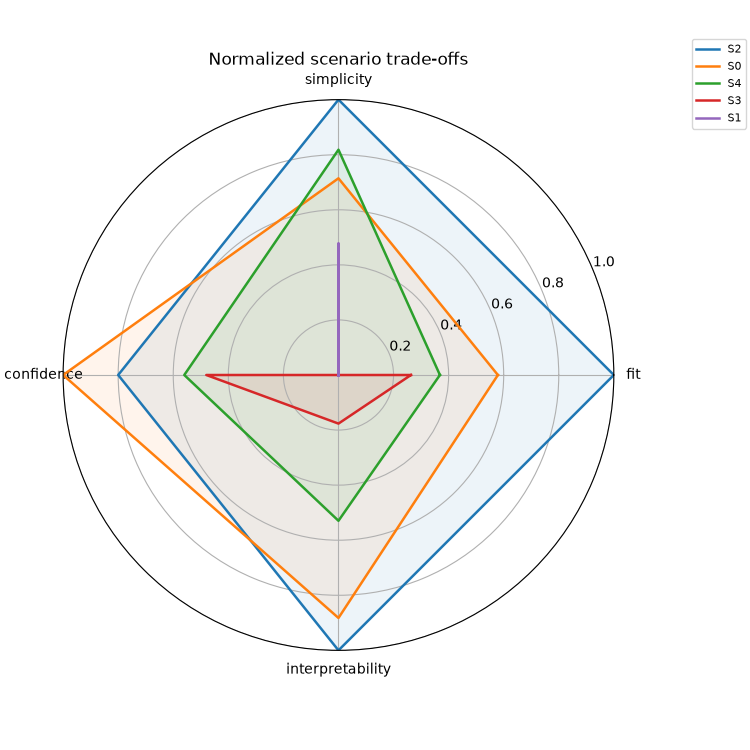
     S2_conservative_errors        0.960000   1.000000          1.000000                         0.80                1.000000
 S0_baseline_corrected_topo        0.757674   0.578947          0.714286                         1.00                0.882353
S4_simple_halfspace_no_topo        0.551375   0.368421          0.818182                         0.56                0.529412
       S3_aggressive_errors        0.223399   0.263158          0.000000                         0.48                0.176471
S1_uncorrected_static_shift        0.120130   0.000000          0.480519                         0.00                0.000000
7. Plot a scenario decision dashboard#
The dashboard separates fit from model complexity. Scenarios in the lower left are usually attractive: lower RMS and lower roughness. Scenarios in the lower right may fit data but can be too complex. Scenarios in the upper left may be simple but underfit.
fig, axes = plt.subplots(2, 2, figsize=(13.0, 9.5), constrained_layout=True)
ax_trade, ax_score, ax_rms, ax_text = axes.ravel()

scatter = ax_trade.scatter(
    scenarios["roughness_proxy"],
    scenarios["final_rms"],
    s=180,
    c=scenarios["processing_confidence"],
    cmap="viridis",
    edgecolor="black",
    linewidth=0.8,
)
for row in scenarios.itertuples(index=False):
    label = row.scenario.split("_", 1)[0]
    ax_trade.annotate(
        label,
        (row.roughness_proxy, row.final_rms),
        xytext=(6, 5),
        textcoords="offset points",
        fontsize=9,
    )
ax_trade.set_xlabel("Roughness / model-complexity proxy")
ax_trade.set_ylabel("Final RMS")
ax_trade.set_title("Fit versus complexity")
ax_trade.grid(alpha=0.25)
cbar = fig.colorbar(scatter, ax=ax_trade, pad=0.01)
cbar.set_label("Processing confidence")

score_plot = scored.sort_values("weighted_score")
ax_score.barh(
    score_plot["scenario"],
    score_plot["weighted_score"],
    color="tab:blue",
    alpha=0.85,
)
ax_score.set_xlabel("Weighted decision score")
ax_score.set_title("Scenario ranking")
ax_score.grid(axis="x", alpha=0.25)

x = np.arange(len(scenarios))
width = 0.35
ax_rms.bar(
    x - width / 2,
    scenarios["final_rms"],
    width=width,
    label="Final RMS",
    color="tab:orange",
)
ax_rms.bar(
    x + width / 2,
    scenarios["best_rms"],
    width=width,
    label="Best RMS",
    color="tab:green",
)
ax_rms.set_xticks(x)
ax_rms.set_xticklabels(
    [name.split("_", 1)[0] for name in scenarios["scenario"]],
)
ax_rms.set_ylabel("RMS")
ax_rms.set_title("Final and best RMS by scenario")
ax_rms.legend()
ax_rms.grid(axis="y", alpha=0.25)

best = scored.iloc[0]
baseline_row = scenarios[
    scenarios["scenario"] == "S0_baseline_corrected_topo"
].iloc[0]
summary_lines = [
    "Decision notes",
    "--------------",
    f"Top-ranked scenario: {best['scenario']}",
    f"Weighted score: {best['weighted_score']:.2f}",
    "",
    "Baseline measured values:",
    f"  final RMS: {baseline_row['final_rms']:.2f}",
    f"  log records: {baseline_stats['n_log_records']}",
    f"  best iteration: {baseline_stats['best_iteration']}",
    "",
    "Do not choose solely by RMS.",
    "Check whether improved fit requires",
    "unreasonable roughness, weak processing",
    "justification, or unstable structures.",
]
ax_text.axis("off")
ax_text.text(
    0.02,
    0.98,
    "\n".join(summary_lines),
    va="top",
    family="monospace",
    fontsize=10,
)

dashboard_file = figure_dir / "inversion_scenario_comparison_dashboard.png"
fig.savefig(dashboard_file, dpi=120)
plt.show()
8. Plot a radar-style trade-off view#
The radar plot is compact for reports because each axis has the same “larger is better” direction after normalization.
radar_metrics = [
    "score_fit",
    "score_simplicity",
    "score_processing_confidence",
    "score_interpretability",
]
radar_labels = ["fit", "simplicity", "confidence", "interpretability"]
angles = np.linspace(0, 2 * np.pi, len(radar_metrics), endpoint=False)
angles = np.concatenate([angles, [angles[0]]])

fig_radar, ax_radar = plt.subplots(
    figsize=(7.5, 7.5),
    subplot_kw={"projection": "polar"},
    constrained_layout=True,
)

for _, row in scored.iterrows():
    values = row[radar_metrics].to_numpy(dtype=float)
    values = np.concatenate([values, [values[0]]])
    ax_radar.plot(
        angles, values, linewidth=1.8, label=row["scenario"].split("_", 1)[0]
    )
    ax_radar.fill(angles, values, alpha=0.08)

ax_radar.set_xticks(angles[:-1])
ax_radar.set_xticklabels(radar_labels)
ax_radar.set_ylim(0.0, 1.0)
ax_radar.set_title("Normalized scenario trade-offs")
ax_radar.legend(loc="upper right", bbox_to_anchor=(1.25, 1.12), fontsize=8)
radar_file = figure_dir / "inversion_scenario_tradeoff_radar.png"
fig_radar.savefig(radar_file, dpi=120)
plt.show()
9. Export a recommendation memo#
The memo is deliberately plain JSON so it can be attached to a report, loaded by a notebook, or compared between project revisions.
recommendation = {
    "recommended_scenario": str(best["scenario"]),
    "reason": (
        "Highest weighted score after balancing data fit, model simplicity, "
        "processing confidence, and interpretability."
    ),
    "weights": weights,
    "baseline_run": str(sample_dir),
    "baseline_stats": baseline_stats,
    "caveats": [
        "Only S0 is a real bundled run in this documentation example.",
        "Replace synthetic what-if rows with real run folders for production.",
        "Always inspect response residuals and section stability before final interpretation.",
    ],
    "outputs": {
        "scenario_table": str(scenario_file),
        "score_table": str(score_file),
        "dashboard": str(dashboard_file),
        "radar": str(radar_file),
    },
}
memo_file = table_dir / "inversion_scenario_recommendation.json"
memo_file.write_text(json.dumps(recommendation, indent=2), encoding="utf-8")

print(f"Scenario table: {scenario_file}")
print(f"Score table: {score_file}")
print(f"Dashboard: {dashboard_file}")
print(f"Radar plot: {radar_file}")
print(f"Recommendation memo: {memo_file}")
Scenario table: /opt/build/repo/docs/examples/inversion/workspaces/modem_result_tables/inversion_scenario_comparison.csv
Score table: /opt/build/repo/docs/examples/inversion/workspaces/modem_result_tables/inversion_scenario_scores.csv
Dashboard: /opt/build/repo/docs/examples/inversion/workspaces/modem_result_figures/inversion_scenario_comparison_dashboard.png
Radar plot: /opt/build/repo/docs/examples/inversion/workspaces/modem_result_figures/inversion_scenario_tradeoff_radar.png
Recommendation memo: /opt/build/repo/docs/examples/inversion/workspaces/modem_result_tables/inversion_scenario_recommendation.json
10. How to adapt this to real run folders#
In a real project, replace the synthetic scenario multipliers with measured values:
result = InversionResult(path_to_each_run)
Then collect:
final/best RMS from
result.log;model roughness or model-change metrics from
result.model_initialandresult.model_final;response residual summaries from the observed/predicted comparison example;
processing metadata such as correction method, topography, mesh, error floors, and starting model.
A final scenario choice should be defendable in words: “we selected this run because it fits the data sufficiently, does not add unnecessary roughness, survives processing sensitivity tests, and keeps the same main geological features across scenarios.”
Total running time of the script: (0 minutes 1.127 seconds)