Inversion#
Classical inversion workflows for pyCSAMT: preparing corrected survey data, building inversion work folders, checking meshes and control files, launching or documenting external inversion runs, and plotting inversion results.
This section is intentionally separate from AI inversion. The AI gallery focuses on neural-network inversion
with pycsamt.ai; this section focuses on practical geophysical
inversion handoff and interpretation, including ModEM/Occam-style workflows
and result diagnostics.
Planned gallery examples#
We will build this section gradually. A useful order is:
Prepare an inversion workspace from corrected EDIs Load a corrected EDI folder, audit station/frequency coverage, choose TE/TM or impedance components, write a clean inversion-ready workspace, and save a processing manifest.
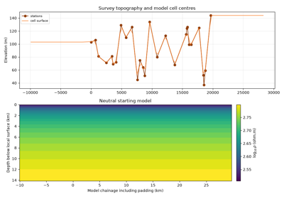
Build a starting model and depth grid Use station spacing, frequency band, skin-depth estimates, and optional topography to propose horizontal cells, vertical layers, padding, and a starting/background resistivity.
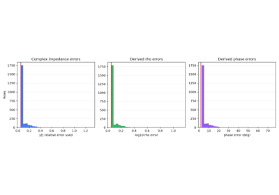
Write inversion data/error tables Convert corrected impedance/phase data into the data table expected by a target inversion backend, with explicit floors for impedance, apparent resistivity, phase, and tipper where available.
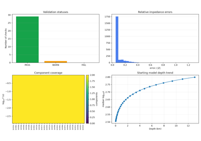
Validate inversion inputs before running Check missing stations, duplicated frequencies, non-finite errors, unrealistic phase ranges, over-aggressive error floors, and whether the selected dimensionality is defensible.
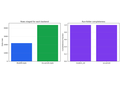
Create a ModEM/Occam-style run folder Assemble data, model, covariance/control files, notes, and launch command metadata without actually requiring the external solver during the docs build.
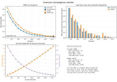
Monitor inversion convergence Parse an inversion log or synthetic run history, plot RMS versus iteration, identify stalls, and explain when to adjust damping, error floors, or mesh design.
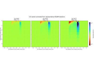
Plot a 2-D inversion section Load a finished result or a lightweight example model, plot resistivity with station markers, topography, DOI/sensitivity overlays, and interpreted conductive/resistive zones.
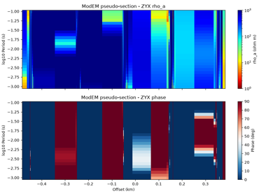
Compare observed and predicted responses Pair measured and model-predicted responses station by station, plot residual pseudo-sections, and identify frequency bands or stations that still control misfit.
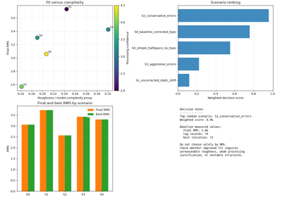
Compare inversion scenarios Compare alternative runs such as raw vs corrected data, different error floors, different starting models, static-shift on/off, or topo on/off.
Prepare the final interpretation package Export section figures, model tables, station metadata, RMS summaries, processing manifests, and caveats suitable for a report or handoff.
The first examples should emphasize reproducible preparation and validation; plotting polished inversion results becomes much more useful once the input contract is clear.
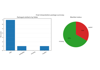

Full inversion case study: from field data to interpretation package
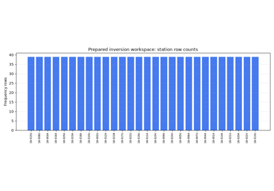
Prepare an inversion workspace from corrected EDIs