2-D section inversion with a U-Net

Moving from 1-D to 2-D, the target is no longer a handful of layer parameters but a full resistivity cross-section — a (depth × station) image. EMInverter2D uses a U-Net, the workhorse image-to-image architecture, to map a pseudo-section of responses to that image in one pass.

To keep the example self-contained and fast, we synthesise training pairs directly: random 2-D resistivity sections (the targets) and a cheap depth→period projection of each as the input “data”. The network never sees the generating rule — it must learn the mapping — so the workflow, API, and validation figures are exactly what you would use with physically-forward-modelled training data.

Synthesise (response → section) training pairs

Each target section is a deepening background with one conductive and one resistive blob at random positions. The input is a (components, freqs, stations) tensor built by averaging the section over depth bands that stand in for period — low frequencies “see” deeper.

import numpy as np

# Use the true/predicted/difference section triptych (2nd figure) as thumb.

N_PROF, N_COMP, N_FREQ, N_STA, N_DEPTH = 90, 2, 18, 28, 28


def make_section(seed):
    r = np.random.default_rng(seed)
    z = np.linspace(0, 1, N_DEPTH)[:, None]
    s = np.linspace(0, 1, N_STA)[None, :]
    section = 1.8 + 0.9 * z + 0.0 * s  # background (D, S)
    # conductive blob (low rho)
    cx, cz = r.uniform(0.2, 0.55), r.uniform(0.25, 0.6)
    section += -0.9 * np.exp(
        -(((s - cx) ** 2) / 0.02 + ((z - cz) ** 2) / 0.03)
    )
    # resistive blob (high rho)
    rx, rz = r.uniform(0.55, 0.85), r.uniform(0.35, 0.75)
    section += 0.7 * np.exp(
        -(((s - rx) ** 2) / 0.02 + ((z - rz) ** 2) / 0.04)
    )
    return section.astype(np.float32)


rng = np.random.default_rng(0)
Y = np.stack([make_section(i) for i in range(N_PROF)])  # (P, D, S)
X = np.zeros((N_PROF, N_COMP, N_FREQ, N_STA), np.float32)
for f in range(N_FREQ):
    d0 = int(f / N_FREQ * N_DEPTH)
    d1 = min(N_DEPTH, d0 + N_DEPTH // N_FREQ + 2)
    band = Y[:, d0:d1, :].mean(axis=1)  # (P, S)
    for c in range(N_COMP):
        X[:, c, f, :] = band + rng.normal(0, 0.03, size=band.shape)

Xtr, Ytr, Xte, Yte = X[:70], Y[:70], X[70:], Y[70:]
print("train:", Xtr.shape, Ytr.shape, " test:", Xte.shape, Yte.shape)

train: (70, 2, 18, 28) (70, 28, 28)  test: (20, 2, 18, 28) (20, 28, 28)

The input data: a pseudo-section

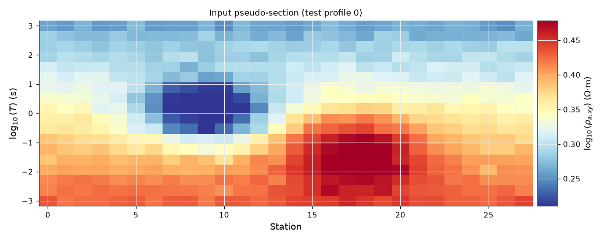
plot_pseudo_section() renders one profile’s input — apparent resistivity across station (x) and frequency (y). This is what the network receives.

from pycsamt.ai.plot import plot_pseudo_section

fig = plot_pseudo_section(
    Xte[0, 0], title="Input pseudo-section (test profile 0)"
)

Train the U-Net and predict

The network shapes are declared up front; fit handles normalisation and the training loop.

import os

from pycsamt.ai.inversion.inv2d import EMInverter2D

# Lighter training while building the docs (PYCSAMT_DOCS_BUILD is set by Sphinx);
# full strength when the example is run directly.
_DOCS = bool(os.environ.get("PYCSAMT_DOCS_BUILD"))

inv = EMInverter2D(
    n_components=N_COMP,
    n_depth=N_DEPTH,
    n_stations=N_STA,
    n_freqs=N_FREQ,
    arch="unet",
)
inv.fit(Xtr, Ytr, epochs=6 if _DOCS else 30, batch_size=8, verbose=False)
pred = np.asarray(inv.predict(Xte))
print("predicted sections:", pred.shape)

predicted sections: (20, 28, 28)

True vs predicted section

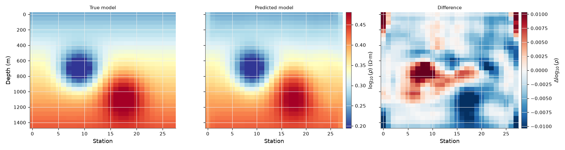
plot_section_pair() shows ground truth, prediction, and their difference side by side. The network recovers both anomalies and the background gradient; the difference panel localises the residual error.

from pycsamt.ai.plot import plot_section, plot_section_pair

fig = plot_section_pair(
    Yte[0], pred[0], depth_max=1500.0, station_spacing=1.0
)

The prediction on its own

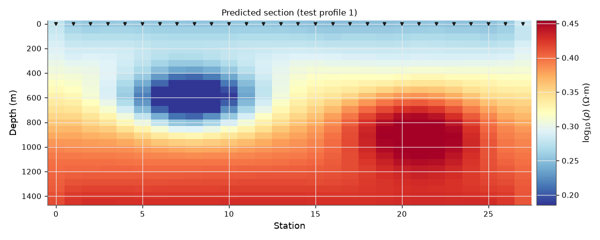
plot_section() draws a single section with the EM resistivity colour map — the figure you would export per profile.

fig = plot_section(
    pred[1], depth_max=1500.0, title="Predicted section (test profile 1)"
)

A grid of held-out profiles

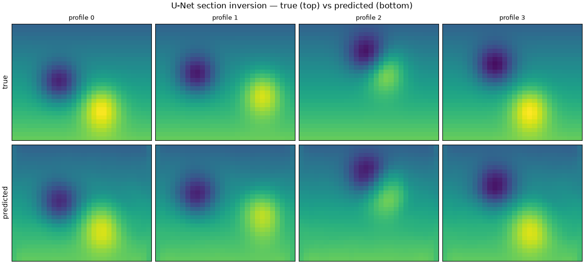
Laying several test profiles out as a true/predicted grid is the quickest way to judge generalisation across the whole test set at a glance.

import matplotlib.pyplot as plt

n_show = 4
fig, axes = plt.subplots(
    2, n_show, figsize=(3.0 * n_show, 5.4), constrained_layout=True
)
vmin, vmax = float(Yte.min()), float(Yte.max())
for k in range(n_show):
    axes[0, k].imshow(
        Yte[k], aspect="auto", cmap="viridis", vmin=vmin, vmax=vmax
    )
    axes[1, k].imshow(
        pred[k], aspect="auto", cmap="viridis", vmin=vmin, vmax=vmax
    )
    axes[0, k].set_title(f"profile {k}", fontsize=9)
    for row in (0, 1):
        axes[row, k].set_xticks([])
        axes[row, k].set_yticks([])
axes[0, 0].set_ylabel("true", fontsize=10)
axes[1, 0].set_ylabel("predicted", fontsize=10)
fig.suptitle(
    r"U-Net section inversion — true (top) vs predicted (bottom)", fontsize=12
)

Text(0.5, 0.9922833333333333, 'U-Net section inversion — true (top) vs predicted (bottom)')

Takeaway. A U-Net inverts a whole 2-D section in a single forward pass. With physically forward-modelled training pairs (see 2-D MT forward models and pseudo-sections) the same pipeline produces field-ready sections. The next example scales up again — to a whole 3-D survey — with a graph network.