3-D survey inversion with a graph network

The largest step: invert an entire multi-station survey at once. Stations are not independent — neighbours see overlapping subsurface — so GCNInverter3D treats the survey as a graph: each station is a node, edges connect nearby stations, and a graph convolutional network (GCN) shares information along those edges while predicting a layered model at every node.

This example generates a pseudo-3-D synthetic survey, builds the station graph, trains the GCN, and validates it with maps, a cross-section, and a Monte-Carlo-dropout uncertainty map.

A pseudo-3-D survey dataset

generate_dataset_3d() draws spatially correlated resistivity fields (a Gaussian random field over the station grid) and forward-models each station. It returns per-survey tensors X (n_stations × features), targets y (n_stations × model params), and the station coords.

import numpy as np

from pycsamt.forward.batch import generate_dataset_3d

# Use the 3-D station-graph context (1st figure) as the thumbnail.

N_LAYERS = 3
ds = generate_dataset_3d(
    solver="mt1d",
    n_surveys=220,
    n_stations=25,
    n_layers=N_LAYERS,
    freqs=np.logspace(-1, 3, 16),
    extent=10_000.0,
    station_layout="grid",
    seed=0,
    verbose=False,
)
print("X:", ds.X.shape, " y:", ds.y.shape, " coords:", ds.coords.shape)
print("features/station:", ds.n_features, " params/station:", ds.y.shape[-1])
train, val, test = ds.split()

X: (220, 25, 32)  y: (220, 25, 5)  coords: (25, 2)
features/station: 32  params/station: 5

Build the station graph

build_adjacency() connects stations within a radius. The adjacency matrix is what lets the GCN pass information between neighbouring soundings — the mechanism that makes it “3-D aware”.

from pycsamt.ai.nets import build_adjacency

RADIUS = 3200.0
A = build_adjacency(ds.coords, radius=RADIUS)
print(
    "adjacency:",
    A.shape,
    " mean neighbours/station:",
    f"{(A > 0).sum(axis=1).mean() - 1:.1f}",
)

adjacency: (25, 25)  mean neighbours/station: 3.2

The graph, in 3-D

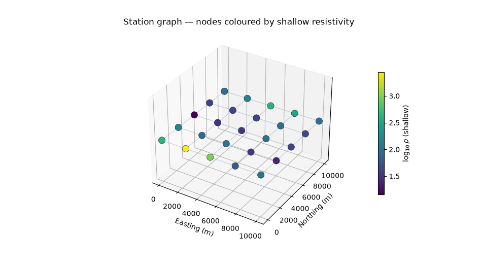
Plotting the stations with their edges shows the context each node draws on. Node colour is the (soon-to-be-predicted) shallow resistivity — the GCN will smooth predictions along these connections.

import matplotlib.pyplot as plt

x, y = ds.coords[:, 0], ds.coords[:, 1]
node_val = test.y[0][:, 0]  # shallow-layer log-rho, survey 0
fig = plt.figure(figsize=(9.5, 5.2))
ax = fig.add_subplot(111, projection="3d")
for i in range(len(x)):
    for j in range(i + 1, len(x)):
        if A[i, j] > 0:
            ax.plot(
                [x[i], x[j]],
                [y[i], y[j]],
                [0, 0],
                color="#94a3b8",
                alpha=0.5,
                lw=0.8,
            )
sc = ax.scatter(
    x,
    y,
    np.zeros_like(x),
    c=node_val,
    cmap="viridis",
    s=90,
    edgecolor="#111827",
    linewidth=0.4,
    depthshade=False,
)
ax.set_xlabel("Easting (m)")
ax.set_ylabel("Northing (m)")
ax.set_zlabel("")
ax.set_zticks([])
ax.set_title("Station graph — nodes coloured by shallow resistivity", pad=10)
ax.view_init(elev=32, azim=-58)
fig.colorbar(
    sc, ax=ax, shrink=0.6, pad=0.1, label=r"$\log_{10}\rho$ (shallow)"
)

<matplotlib.colorbar.Colorbar object at 0x7f2aaafbf3e0>

Train the GCN and predict

fit accepts either a prebuilt adjacency or raw coords + a radius. Training is fast because the whole survey is one graph.

import os

from pycsamt.ai.inversion.inv3d import GCNInverter3D

# Lighter training while building the docs (PYCSAMT_DOCS_BUILD is set by Sphinx);
# full strength when the example is run directly.
_DOCS = bool(os.environ.get("PYCSAMT_DOCS_BUILD"))

inv = GCNInverter3D(n_features=ds.n_features, n_layers=N_LAYERS, hidden=(64,))
inv.fit(
    train.X,
    train.y,
    coords=ds.coords,
    radius=RADIUS,
    epochs=12 if _DOCS else 60,
    verbose=False,
)
pred = inv.predict(test.X)  # (n_test, n_stations, n_out)
print("predicted survey tensor:", pred.shape)

predicted survey tensor: (22, 25, 5)

Predicted vs true resistivity map

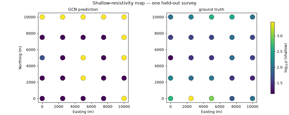
For one held-out survey, map the shallow-layer resistivity across the station grid: prediction (left) against truth (right). The GCN reproduces the spatial pattern, not just per-station values.

survey = 0
true0, pred0 = test.y[survey], pred[survey]
fig, (axp, axt) = plt.subplots(
    1, 2, figsize=(11, 4.4), constrained_layout=True
)
vmin, vmax = float(true0[:, 0].min()), float(true0[:, 0].max())
for ax, val, ttl in [
    (axp, pred0[:, 0], "GCN prediction"),
    (axt, true0[:, 0], "ground truth"),
]:
    s = ax.scatter(
        x,
        y,
        c=val,
        cmap="viridis",
        s=180,
        vmin=vmin,
        vmax=vmax,
        edgecolor="#111827",
        linewidth=0.4,
    )
    ax.set_title(ttl, fontsize=11)
    ax.set_xlabel("Easting (m)")
    ax.set_aspect("equal")
axp.set_ylabel("Northing (m)")
fig.colorbar(s, ax=[axp, axt], shrink=0.8, label=r"$\log_{10}\rho$ (shallow)")
fig.suptitle("Shallow-resistivity map — one held-out survey", fontsize=12)

Text(0.5, 0.9905295454545454, 'Shallow-resistivity map — one held-out survey')

A cross-section through the survey

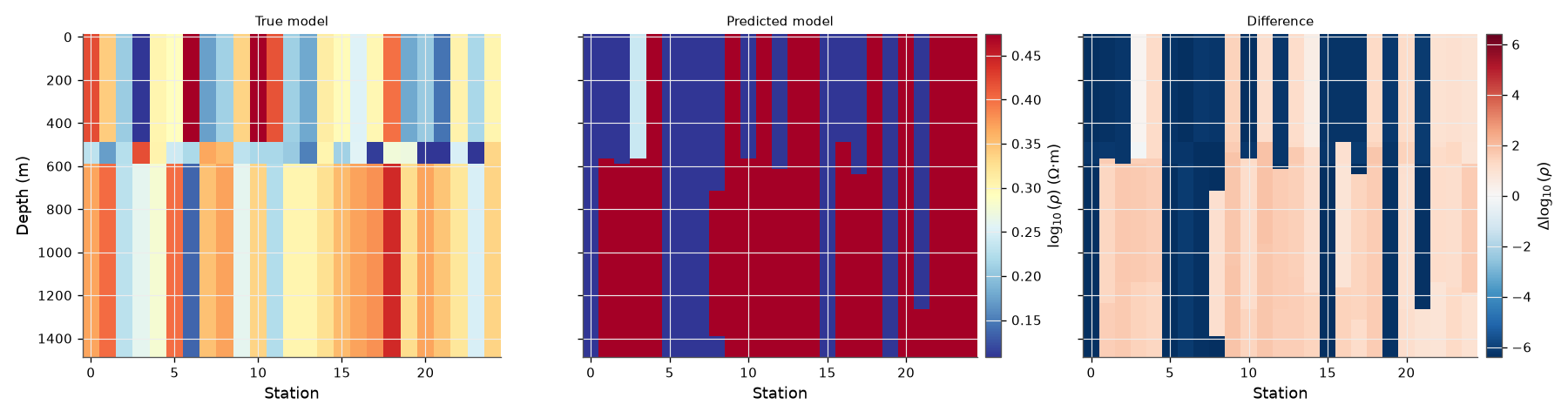
Expanding every station’s predicted layer model onto a depth axis (ordered by easting) turns the node predictions into a resistivity cross-section, comparable to the classical and 2-D outputs.

from pycsamt.ai.plot import plot_section_pair


def survey_section(param_grid, depth_max=1500.0, n=60):
    """(n_stations, 2L-1) params -> (depth, n_stations) log-rho section."""
    order = np.argsort(x)
    depths = np.linspace(0, depth_max, n)
    sec = np.empty((n, len(order)))
    for col, sta in enumerate(order):
        row = param_grid[sta]
        logrho = row[:N_LAYERS]
        thick = np.maximum(row[N_LAYERS:], 1.0)  # thickness is in metres
        edges = np.concatenate([[0.0], np.cumsum(thick), [np.inf]])
        for i in range(N_LAYERS):
            sec[(depths >= edges[i]) & (depths < edges[i + 1]), col] = logrho[
                i
            ]
    return sec


fig = plot_section_pair(
    survey_section(true0), survey_section(pred0), depth_max=1500.0
)

Where is the GCN unsure? An uncertainty map

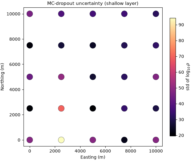
predict_with_uncertainty() runs Monte-Carlo dropout to get a per-station spread. Uncertainty is highest at the survey edges, where each node has fewer graph neighbours to borrow strength from.

mean_u, std_u = inv.predict_with_uncertainty(
    test.X[survey : survey + 1], n_mc=20
)
unc = std_u[0][:, 0]  # shallow-layer std
fig, ax = plt.subplots(figsize=(6.2, 5.2), constrained_layout=True)
s = ax.scatter(
    x, y, c=unc, cmap="magma", s=200, edgecolor="#111827", linewidth=0.4
)
ax.set_xlabel("Easting (m)")
ax.set_ylabel("Northing (m)")
ax.set_aspect("equal")
ax.set_title("MC-dropout uncertainty (shallow layer)", fontsize=11)
fig.colorbar(s, ax=ax, shrink=0.85, label=r"std of $\log_{10}\rho$")

<matplotlib.colorbar.Colorbar object at 0x7f2ac1a8cc20>

Takeaway. A graph network inverts a whole survey jointly, exploiting station geometry that per-sounding 1-D inversion ignores — and the same predict_with_uncertainty interface flags where to trust the result. Together with the 1-D and 2-D examples, this completes the AI-inversion ladder from a single sounding to a full 3-D survey.