Pre-inversion case study: from collected EDIs to corrected EDIs

This case study is written for the common moment after field acquisition:

you have a folder of collected EDI files, and you need to process, correct, document, and export a clean dataset before inversion.

The workflow is deliberately complete. It does not jump straight to a final plot. It moves through the same decisions an interpreter should record in a processing notebook:

1. load the collected line and audit station/frequency coverage;

2. select the inversion band and remove low-confidence frequencies;

3. correct frequency-independent static shift;

4. apply confidence-gated spatial EMAP conditioning;

5. rotate onto strike and antisymmetrise for 2-D inversion;

6. compare raw and final tensors;

7. export corrected EDIs and reload them as a final sanity check.

The example uses the bundled WILLY L18PLT line, but the path can be replaced by a survey folder collected by a user.

1. Imports and project paths

Gallery examples are meant to be copied. Keep imports at the top and use public package-level imports where possible.

import os
import sys
from pathlib import Path

# sphinx-gallery executes examples without __file__ (the gallery
# runner sets the working directory to this example's folder).
try:
    EXAMPLE_DIR = Path(__file__).resolve().parent
except NameError:
    EXAMPLE_DIR = Path.cwd()

import matplotlib.pyplot as plt
import numpy as np


def repo_root():
    root = os.environ.get("PYCSAMT_DOCS_REPO_ROOT")
    return Path(root) if root else EXAMPLE_DIR.parents[2]


ROOT = repo_root()
if str(ROOT) not in sys.path:
    sys.path.insert(0, str(ROOT))

from pycsamt.emtools import (
    antisymmetrize,
    confidence_gated_emap_filter,
    correct_ss_ama,
    drop_duplicates,
    edit_frequencies_by_confidence,
    ensure_sites,
    plot_emap_filter_psection,
    plot_frequency_edit_decisions,
    plot_frequency_edit_summary,
    plot_ss_summary,
    plot_strike_profile,
    rotate_to_strike,
    select_band,
)
from pycsamt.emtools._core import _get_z_block, _iter_items, _name
from pycsamt.site import SitesReport, write_sites

raw_dir = ROOT / "data" / "AMT" / "WILLY_DATA" / "L18PLT"
export_dir = EXAMPLE_DIR / "edi_out" / "pre_inversion_l18"

2. Load the collected EDI folder

ensure_sites is the canonical loader. Use recursive=False when the survey folder contains only one line; use recursive=True for nested field folders.

raw = ensure_sites(raw_dir, recursive=False, verbose=0)
raw_report = SitesReport(raw).to_dataframe(api=False)

print("Collected EDI folder:", raw_dir)
print(f"Stations loaded: {len(raw_report)}")
print(
    "Frequency rows per station: "
    f"{raw_report['nfreq'].min()}-{raw_report['nfreq'].max()}"
)
print("First stations:")
print(
    raw_report[["station", "nfreq", "lat", "lon", "elev"]]
    .head()
    .to_string(index=False)
)

Collected EDI folder: /opt/build/repo/data/AMT/WILLY_DATA/L18PLT
Stations loaded: 28
Frequency rows per station: 53-53
First stations:
station  nfreq       lat        lon  elev
18-015U     53 32.132933 119.128750 103.0
18-008U     53 32.126617 119.128800 106.0
18-003A     53 32.122083 119.128850  81.0
18-016A     53 32.133817 119.128767  71.0
18-025A     53 32.141950 119.129017  81.0

3. Small utility functions for tensor-level diagnostics

Some correction steps change the frequency grid. Reading diagnostics directly from Z.z avoids relying on cached apparent-resistivity arrays that may belong to the pre-edit grid in older containers.

def z_component_curves(sites, component="xy"):
    ij = {"xx": (0, 0), "xy": (0, 1), "yx": (1, 0), "yy": (1, 1)}[component]
    out = {}
    for i, ed in enumerate(_iter_items(sites)):
        _Z, z, fr = _get_z_block(ed)
        if z is None or fr is None:
            continue
        period = 1.0 / np.asarray(fr, dtype=float)
        out[_name(ed, i)] = (period, np.abs(np.asarray(z)[:, ij[0], ij[1]]))
    return out


def finite_row_counts(sites):
    rows = []
    for i, ed in enumerate(_iter_items(sites)):
        _Z, z, fr = _get_z_block(ed)
        if z is None or fr is None:
            rows.append((_name(ed, i), 0, 0))
            continue
        finite = np.isfinite(np.asarray(z).reshape(len(fr), -1)).all(axis=1)
        rows.append((_name(ed, i), len(fr), int(finite.sum())))
    return rows


def diagonal_ratio(sites):
    values = []
    labels = []
    for i, ed in enumerate(_iter_items(sites)):
        _Z, z, _fr = _get_z_block(ed)
        if z is None:
            continue
        z = np.asarray(z)
        diag = np.sqrt(np.abs(z[:, 0, 0]) ** 2 + np.abs(z[:, 1, 1]) ** 2)
        off = np.sqrt(np.abs(z[:, 0, 1]) ** 2 + np.abs(z[:, 1, 0]) ** 2)
        labels.append(_name(ed, i))
        values.append(float(np.nanmedian(diag / np.maximum(off, 1e-24))))
    return labels, np.asarray(values, dtype=float)


def z_logmag_matrix(sites, component="xy"):
    ij = {"xx": (0, 0), "xy": (0, 1), "yx": (1, 0), "yy": (1, 1)}[component]
    labels = []
    grids = []
    values = []
    for i, ed in enumerate(_iter_items(sites)):
        _Z, z, fr = _get_z_block(ed)
        if z is None or fr is None:
            continue
        labels.append(_name(ed, i))
        grids.append(np.asarray(fr, dtype=float))
        values.append(
            np.log10(np.abs(np.asarray(z)[:, ij[0], ij[1]]) + 1e-24)
        )
    if not values:
        return [], np.array([], dtype=float), np.empty((0, 0), dtype=float)
    common = np.sort(np.unique(np.concatenate(grids)))
    matrix = np.full((len(values), len(common)), np.nan, dtype=float)
    for row, (grid, vals) in enumerate(zip(grids, values)):
        for col, freq in enumerate(common):
            idx = int(np.nanargmin(np.abs(grid - freq)))
            if np.isclose(grid[idx], freq, rtol=1e-6, atol=1e-12):
                matrix[row, col] = vals[idx]
    return labels, common, matrix


def plot_curve_compare(before, after, stations, *, title, after_label, color):
    fig, axes = plt.subplots(
        1,
        len(stations),
        figsize=(4.0 * len(stations), 4.2),
        sharey=True,
        constrained_layout=True,
    )
    if len(stations) == 1:
        axes = [axes]
    for ax, station in zip(axes, stations):
        pb, vb = before[station]
        pa, va = after[station]
        ax.loglog(pb, vb, ".", ms=3, color="#a8a29e", label="collected")
        ax.loglog(pa, va, "-", lw=1.7, color=color, label=after_label)
        ax.set_title(station, fontsize=9)
        ax.set_xlabel("period (s)")
        ax.grid(True, which="both", ls=":", lw=0.4, alpha=0.6)
    axes[0].set_ylabel(r"$|Z_{xy}|$")
    axes[0].legend(fontsize=8)
    fig.suptitle(title, fontsize=12)
    return fig

4. Define processing targets before changing the data

Record the policy first. In a real project these numbers belong in the processing report, because they explain why the final EDI files differ from the collected files.

fmin_hz = 1e-3
fmax_hz = 1e3
ci_hi = 0.90
ci_lo = 0.62
emap_window = 5
emap_component = "xy"

print("Processing policy:")
print(f"  inversion band: {fmin_hz:g}-{fmax_hz:g} Hz")
print(f"  confidence thresholds: ci_lo={ci_lo}, ci_hi={ci_hi}")
print(f"  gated EMAP: trimmed moving average, window={emap_window}")

Processing policy:
  inversion band: 0.001-1000 Hz
  confidence thresholds: ci_lo=0.62, ci_hi=0.9
  gated EMAP: trimmed moving average, window=5

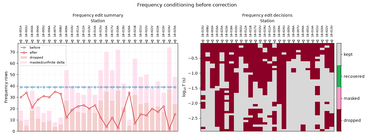
5. Frequency conditioning

The first correction stage makes the line numerically consistent:

• remove duplicate frequency rows;

• keep only the intended inversion band;

• drop rows below the minimum confidence threshold.

We keep an independent raw object for all before/after reporting.

s1 = drop_duplicates(raw_dir, recursive=False)
s2 = select_band(s1, fmin=fmin_hz, fmax=fmax_hz, recursive=False)
freq_edit = edit_frequencies_by_confidence(
    s2,
    before_sites=s2,
    mode="drop",
    method="composite",
    threshold=ci_lo,
    ci_hi=ci_hi,
    ci_lo=ci_lo,
    also="z",
    recursive=False,
)
s3 = freq_edit.sites

print(freq_edit.summary())
print("Frequency-edit decisions:")
print(freq_edit.decisions["action"].value_counts(dropna=False).to_string())

fig, axs = plt.subplots(1, 2, figsize=(13.0, 4.8))
plot_frequency_edit_summary(
    s2, s3, method="composite", ci_hi=ci_hi, ci_lo=ci_lo, ax=axs[0]
)
plot_frequency_edit_decisions(
    s2, s3, method="composite", ci_hi=ci_hi, ci_lo=ci_lo, ax=axs[1]
)
fig.suptitle("Frequency conditioning before correction", fontsize=12)
fig.tight_layout()

APIResult(name='frequency_edit', kind='emtools.frequency.edit', keys=tuple(len=12, sample=['sites', 'report', 'decisions', ...]))
Frequency-edit decisions:
action
kept       556
dropped    536

6. Static-shift correction

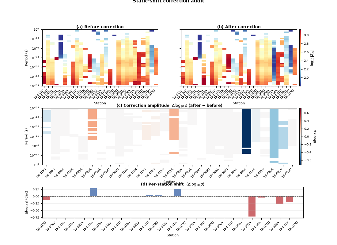
Static shift is a station-wise, frequency-independent amplitude distortion. Correct it before shape-based smoothing or inversion. The AMA method estimates local spatial trends and applies finite positive impedance factors.

s4 = correct_ss_ama(s3, recursive=False)

labels_ss, freqs_ss, before_ss = z_logmag_matrix(s3, component="xy")
_labels_ss_after, _freqs_ss_after, after_ss = z_logmag_matrix(
    s4, component="xy"
)

fig = plot_ss_summary(
    before_ss,
    after_ss,
    freqs=freqs_ss,
    station_labels=labels_ss,
    colorbar_label=r"$\log_{10}|Z_{xy}|$",
    suptitle="Static-shift correction audit",
    figsize=(11.0, 8.0),
)

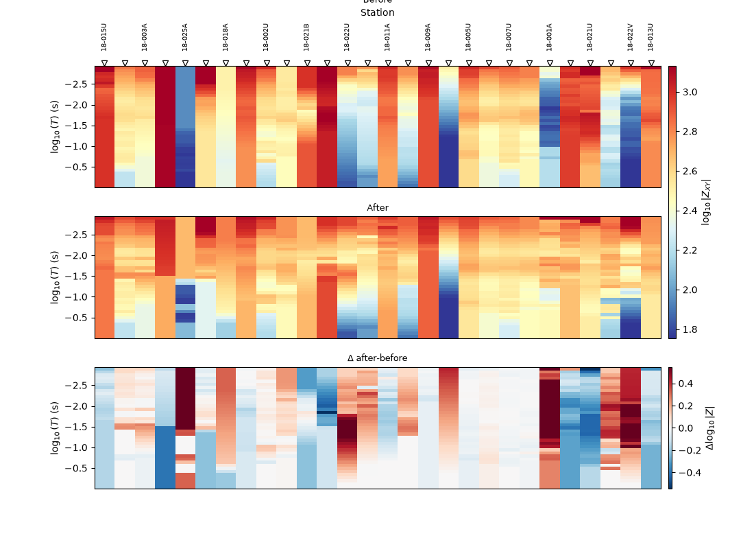
7. Confidence-gated EMAP conditioning

A full EMAP filter can over-smooth good data. The gated filter uses the confidence score to decide how strongly each station-frequency row should follow the spatially filtered estimate.

emap = confidence_gated_emap_filter(
    s4,
    before_sites=s4,
    method="tma",
    confidence_method="composite",
    component=emap_component,
    ci_hi=ci_hi,
    ci_lo=ci_lo,
    blend_power=1.3,
    window=emap_window,
    recursive=False,
)
s5 = emap.sites

print(emap.summary())
print("EMAP actions:")
print(emap.decisions["action"].value_counts(dropna=False).to_string())
print("EMAP report:")
print(emap.report.head(8).to_string(index=False))

plot_emap_filter_psection(
    s4,
    s5,
    method="tma",
    component=emap_component,
    window=emap_window,
    station_label_step=2,
    figsize=(11.0, 8.0),
)

EMAPFilterResult(method='tma', confidence='composite', preserved=0, blended=487, filtered=69)
EMAP actions:
action
blended     487
filtered     69
EMAP report:
station  n_freq  n_preserved  n_blended  n_filtered  mean_blend_weight  median_confidence  median_delta_log10_abs_z
18-015U      12            0         12           0           0.649131           0.699112                 -0.115497
18-008U      33            0         33           0           0.658023           0.715782                  0.013875
18-003A      21            0         20           1           0.592941           0.715387                  0.035671
18-016A       4            0          4           0           0.890212           0.633898                 -0.165974
18-025A      15            0         15           0           0.716535           0.687852                  0.000000
18-023A      17            0         16           1           0.680900           0.704894                 -0.022925
18-018A       3            0          0           3           1.000000           0.540990                  0.149812
18-010U      19            0         18           1           0.466946           0.741749                 -0.073263

<Figure size 1100x800 with 5 Axes>

8. Strike rotation and 2-D tensor preparation

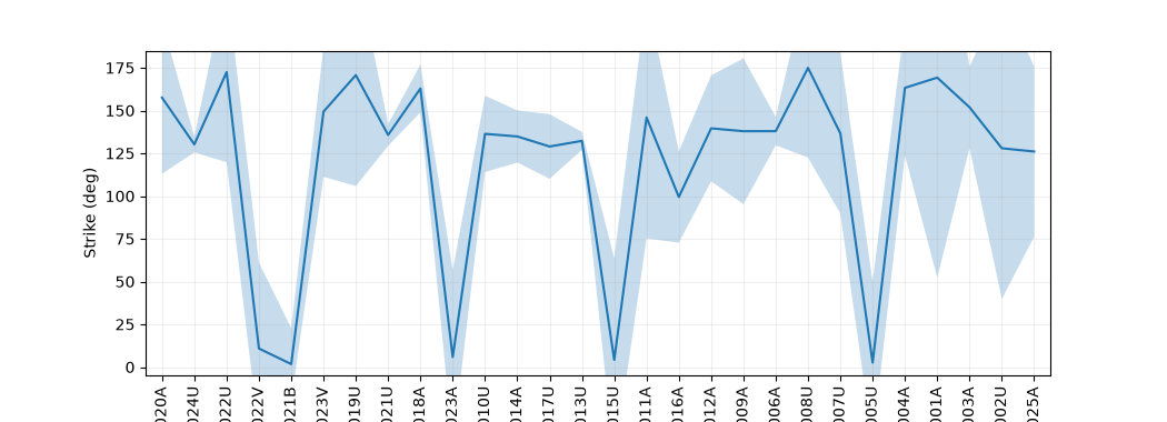
Before 2-D inversion, the tensor should be expressed in an appropriate geoelectric frame. Then, if the target inversion code assumes an ideal 2-D tensor, antisymmetrise the off-diagonal terms.

plot_strike_profile(s5, method="consensus", figsize=(10.5, 3.8))

s6 = rotate_to_strike(s5, recursive=False)
final = antisymmetrize(s6, recursive=False)

labels_raw, ratio_raw = diagonal_ratio(raw)
labels_final, ratio_final = diagonal_ratio(final)
shared = [name for name in labels_raw if name in set(labels_final)]
idx_raw = [labels_raw.index(name) for name in shared]
idx_final = [labels_final.index(name) for name in shared]

fig, ax = plt.subplots(figsize=(11.0, 4.0))
x = np.arange(len(shared))
ax.plot(x, ratio_raw[idx_raw], "o-", color="#a8a29e", label="collected")
ax.plot(
    x, ratio_final[idx_final], "o-", color="#16a34a", label="pre-inversion"
)
ax.set_xticks(x)
ax.set_xticklabels(shared, rotation=90, fontsize=7)
ax.set_ylabel("median diagonal/off-diagonal ratio")
ax.set_title("Tensor 2-D readiness check")
ax.grid(alpha=0.25)
ax.legend()
fig.tight_layout()

print(
    "Median diagonal/off-diagonal ratio: "
    f"{np.nanmedian(ratio_raw):.3f} -> {np.nanmedian(ratio_final):.3f}"
)

• 
• 

/opt/build/repo/pycsamt/z/utils.py:396: ComplexWarning: Casting complex values to real discards the imaginary part
  E = ensure_z3(z_err).astype(float, copy=False)
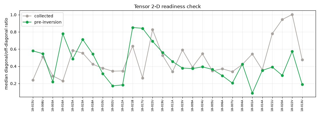
Median diagonal/off-diagonal ratio: 0.423 -> 0.393

9. Raw versus final sounding curves

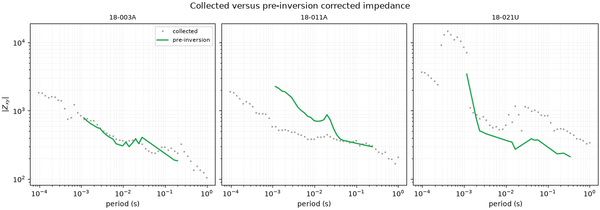
A final curve comparison should show controlled changes, not a mysterious rewrite of the survey. Large changes should correspond to documented frequency edits, static-shift factors, or gated EMAP decisions.

raw_curves = z_component_curves(raw, component="xy")
final_curves = z_component_curves(final, component="xy")
stations = list(raw_curves)
pick = [stations[2], stations[len(stations) // 2], stations[-4]]

plot_curve_compare(
    raw_curves,
    final_curves,
    pick,
    title="Collected versus pre-inversion corrected impedance",
    after_label="pre-inversion",
    color="#16a34a",
)

<Figure size 1200x420 with 3 Axes>

10. Export corrected EDIs and reload them

Export is not just an output step; it is a validation step. If the exported folder cannot be reloaded as impedance-bearing sites, the inversion handoff is not ready.

paths = write_sites(final, export_dir, exist_ok=True)
reloaded = ensure_sites(export_dir, recursive=False, verbose=0)
reload_report = SitesReport(reloaded).to_dataframe(api=False)

print(f"Exported corrected EDIs: {len(paths)}")
print("Export folder:", export_dir)
print(f"Reloaded stations: {len(reload_report)}")
print(
    "Reloaded frequency rows: "
    f"{reload_report['nfreq'].min()}-{reload_report['nfreq'].max()}"
)

if len(reload_report) != len(raw_report):
    raise RuntimeError("Export sanity check failed: station count changed.")

Exported corrected EDIs: 28
Export folder: /opt/build/repo/docs/examples/corrections/edi_out/pre_inversion_l18
Reloaded stations: 28
Reloaded frequency rows: 2-35

11. Final pre-inversion checklist

Before starting inversion, keep these artefacts with the project:

• raw station summary;

• frequency-edit decision table;

• static-shift summary figure;

• gated EMAP decision table;

• strike profile;

• raw-vs-final curve comparison;

• exported EDI folder and reload summary.

The final EDIs are now ready for a 2-D inversion workflow, subject to the geophysical assumptions checked above: acceptable dimensionality, defensible strike, and no unresolved source or near-surface effects.