
Note
Go to the end to download the full example code.
Static-shift correction#
Static shift is the classic MT/AMT distortion: near-surface heterogeneity
multiplies a station’s whole apparent-resistivity curve by a
frequency-independent factor, shifting it vertically without changing its
shape. Left uncorrected it maps straight into a wrong inversion depth.
pycsamt.emtools estimates and removes it two ways — a spatial
array-moving-average (AMA) and the Hanning-EMAP filter.
Estimate the shift#
estimate_ss_ama() estimates the per-station
multiplier without changing the data — spatially averaging log(ρa)
across neighbouring stations (skew-gated so 3-D stations don’t corrupt the
average) and reading each station’s departure from that smooth trend.
import numpy as np
from _corr_data import curves, demo_line, plot_before_after

from pycsamt.emtools import (
    correct_ss_ama,
    correct_static_shift,
    estimate_ss_ama,
)

S = demo_line("L18PLT")
raw = curves(S, "rho")
print(f"{len(raw)} stations on line L18PLT")

est = estimate_ss_ama(S, recursive=False)
print("estimate_ss_ama ->", type(est).__name__)
print(est)
28 stations on line L18PLT
estimate_ss_ama -> APIFrame
APIFrame: estimate_ss_ama
kind: emtools.ss.ama
shape: 28 rows x 5 columns
columns: station, delta_log10_rho, fac_rho, fac_z, n_used
numeric: 4 columns
missing: 0.0%
source: Sites()
description: AMA static-shift correction factors by station.
Correct with the spatial AMA#
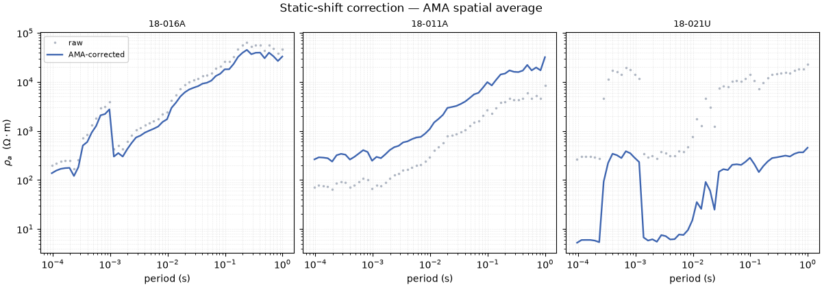
correct_ss_ama() applies that estimate: it divides
each station’s ρa by its multiplier so the curves collapse back
onto the coherent regional trend. The shape (and phase) is untouched — only
the vertical offset is removed.
<Figure size 1200x420 with 3 Axes>
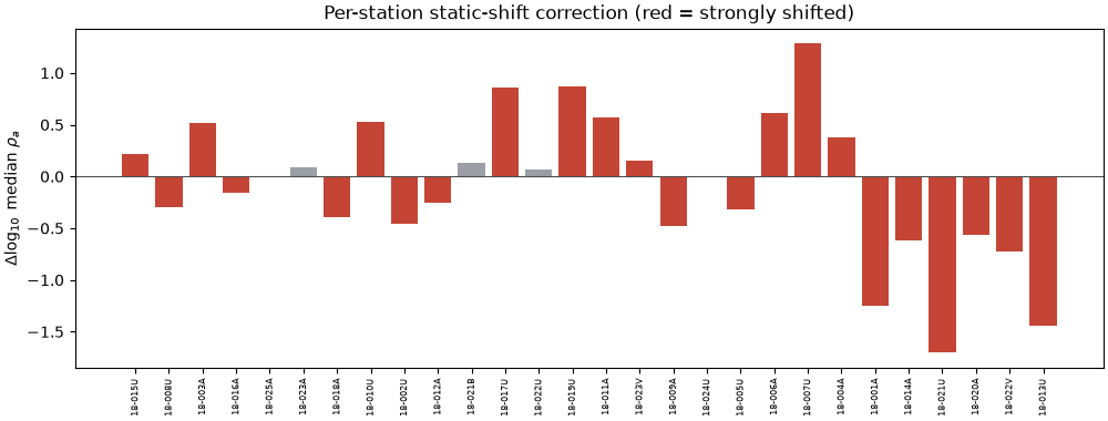
How big was the shift, per station?#
Reducing each station to its median ρa before and after shows the correction as a vertical move — large moves flag the statically-shifted stations, the rest barely change.
import matplotlib.pyplot as plt

med_before = np.array([np.nanmedian(raw[s][1]) for s in stations])
med_after = np.array([np.nanmedian(ama[s][1]) for s in stations])
shift = np.log10(med_after) - np.log10(med_before)
x = np.arange(len(stations))
fig, ax = plt.subplots(figsize=(10, 3.8), constrained_layout=True)
ax.bar(x, shift, color=np.where(np.abs(shift) > 0.15, "#c44536", "#9aa0a6"))
ax.axhline(0, color="0.3", lw=0.8)
ax.set_xticks(x)
ax.set_xticklabels(stations, rotation=90, fontsize=6)
ax.set_ylabel(r"$\Delta\log_{10}$ median $\rho_a$")
ax.set_title("Per-station static-shift correction (red = strongly shifted)")
Text(0.5, 1.0, 'Per-station static-shift correction (red = strongly shifted)')
The Hanning-EMAP alternative#
correct_static_shift() implements the
Torres-Verdín EMAP filter: a Hanning-windowed spatial average of the
log(ρa) profile at each frequency. It uses a physical window
length (metres) rather than a neighbour count, so it adapts to irregular
station spacing. Comparing the two corrected curves is the standard check
that the correction is robust to method choice.
S_emap = correct_static_shift(
    S, window_m=1500.0, spacing_m=200.0, recursive=False
)
emap = curves(S_emap, "rho")

st = pick[1]
fig, ax = plt.subplots(figsize=(6.5, 5.0), constrained_layout=True)
ax.loglog(raw[st][0], raw[st][1], ".", ms=5, color="0.6", label="raw")
ax.loglog(ama[st][0], ama[st][1], "-", lw=1.8, color="#3e65b0", label="AMA")
ax.loglog(
    emap[st][0],
    emap[st][1],
    "--",
    lw=1.8,
    color="#16a34a",
    label="Hanning EMAP",
)
ax.set_xlabel("period (s)")
ax.set_ylabel(r"$\rho_a$  ($\Omega\cdot$m)")
ax.set_title(f"AMA vs Hanning-EMAP at {st}")
ax.legend(fontsize=9)
ax.grid(True, which="both", ls=":", lw=0.4, alpha=0.6)
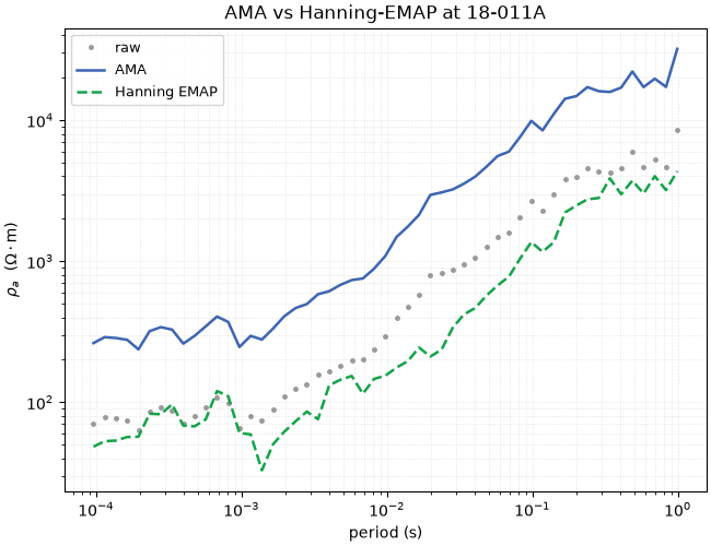
Takeaway. Both methods pull the shifted curves back onto the regional trend while preserving curve shape and phase; where they agree, the correction is trustworthy. Static shift is usually the first wave — run it before the shape-based corrections in noise removal and tensor rotation.
Total running time of the script: (0 minutes 1.306 seconds)