Noise removal

Once the vertical offset is gone, the next wave cleans the shape of each sounding: power-line harmonics, high-frequency scatter, and rough ρ/φ curves. pycsamt.emtools provides a targeted notch, a spectral smoother, and a robust trend smoother — apply them in that order, lightest touch first.

Power-line notch

notch_powerline() suppresses the mains frequency and its harmonics (50 or 60 Hz) by interpolating across the affected bins. On a clean AMT line with no energy at those exact frequencies it is a safe no-op — which is exactly what you want: it only ever touches the harmonic bins, so running it can never hurt.

import numpy as np
from _corr_data import curves, demo_line, plot_before_after

from pycsamt.emtools import (
    notch_powerline,
    smooth_logfreq,
    smooth_rho_phase,
)

S = demo_line("L18PLT")
raw = curves(S, "rho")
S_notch = notch_powerline(S, mains_hz=50.0, n_harm=30, recursive=False)
notch = curves(S_notch, "rho")
changed = sum(
    not np.allclose(raw[s][1], notch[s][1], equal_nan=True) for s in raw
)
print(
    f"notch_powerline changed {changed}/{len(raw)} stations "
    f"(0 = no mains energy in band, as expected for AMT)"
)

notch_powerline changed 0/28 stations (0 = no mains energy in band, as expected for AMT)

Log-frequency smoothing

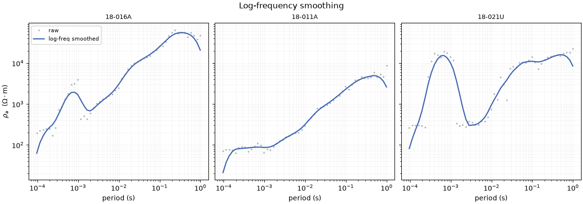
smooth_logfreq() runs a triangular kernel along the log-frequency axis, damping bin-to-bin scatter while preserving the broad spectral shape. This is the workhorse denoiser for ragged curves.

S_sf = smooth_logfreq(S, win=5, kind="tri", recursive=False)
sf = curves(S_sf, "rho")

stations = list(raw)
pick = [stations[3], stations[len(stations) // 2], stations[-4]]
plot_before_after(
    raw,
    sf,
    pick,
    quantity="rho",
    labels=("raw", "log-freq smoothed"),
    title="Log-frequency smoothing",
)

<Figure size 1200x420 with 3 Axes>

Robust ρ/φ trend smoothing

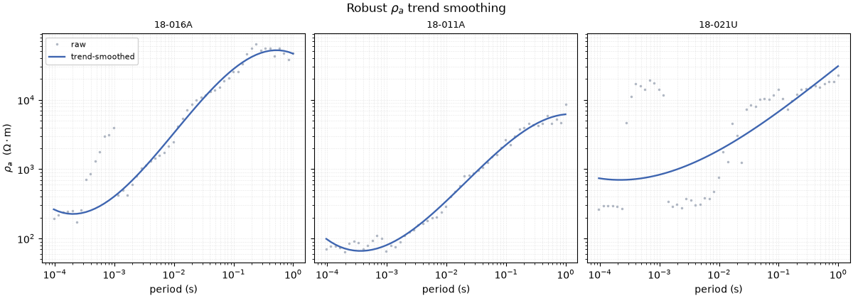
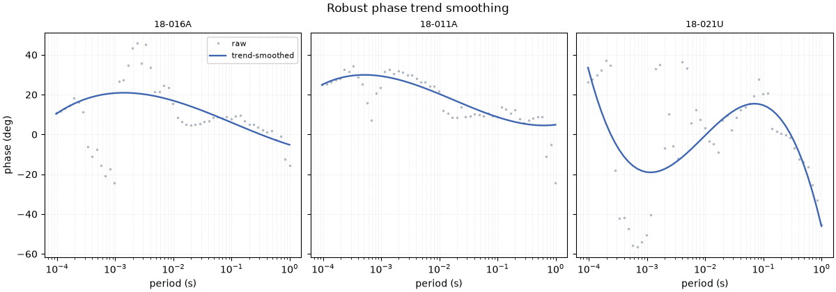
smooth_rho_phase() fits a robust (spike-resistant) low-order polynomial to the log(ρ_a) and phase curves, replacing noisy points with the smooth trend. Because it is robust, isolated outliers are ignored rather than smeared. Here it is applied to the off-diagonal components, shown for both ρ and φ.

S_rp = smooth_rho_phase(
    S, components="offdiag", degree=3, robust=True, recursive=False
)
rp_rho = curves(S_rp, "rho")
rp_phase = curves(S_rp, "phase")
raw_phase = curves(S, "phase")

plot_before_after(
    raw,
    rp_rho,
    pick,
    quantity="rho",
    labels=("raw", "trend-smoothed"),
    title=r"Robust $\rho_a$ trend smoothing",
)

<Figure size 1200x420 with 3 Axes>

… and the matching phase

The same fit cleans the phase, which feeds the inversion just as strongly as resistivity.

plot_before_after(
    raw_phase,
    rp_phase,
    pick,
    quantity="phase",
    labels=("raw", "trend-smoothed"),
    title="Robust phase trend smoothing",
)

<Figure size 1200x420 with 3 Axes>

Takeaway. Notch first (harmless, targeted), then smooth in log-frequency, then apply the robust ρ/φ trend fit for the cleanest inversion-ready curves — always checking that smoothing damps noise without flattening real structure. Next, source effects handles the CSAMT-specific distortions.