Tensor rotation

A 2-D inversion assumes the measurement axes lie along and across the geoelectric strike. Real surveys rarely do, so the final conditioning wave rotates the impedance tensor onto strike and, optionally, antisymmetrises it to enforce the ideal 2-D form. pycsamt.emtools estimates the strike, rotates to it, and prepares the tensor for inversion.

Estimate the geoelectric strike

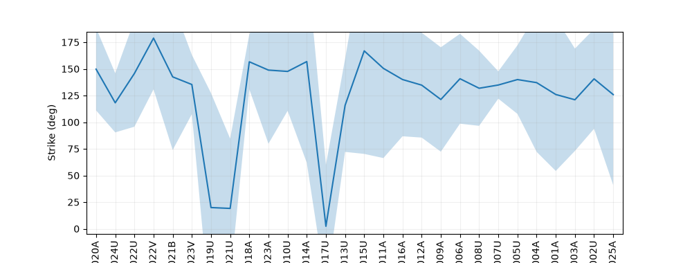
plot_strike_profile() shows the estimated strike along the line (median ± spread), the angle every station will be rotated by. A consistent strike is what makes a 2-D interpretation defensible.

import numpy as np
from _corr_data import curves, demo_line, plot_before_after

from pycsamt.emtools import (
    antisymmetrize,
    plot_strike_profile,
    rotate_to_strike,
)
from pycsamt.emtools._core import _iter_items

S = demo_line("L18PLT")
raw = curves(S, "rho")
plot_strike_profile(S, method="consensus", figsize=(10, 3.8))

<Axes: xlabel='Station', ylabel='Strike (deg)'>

Rotate onto strike

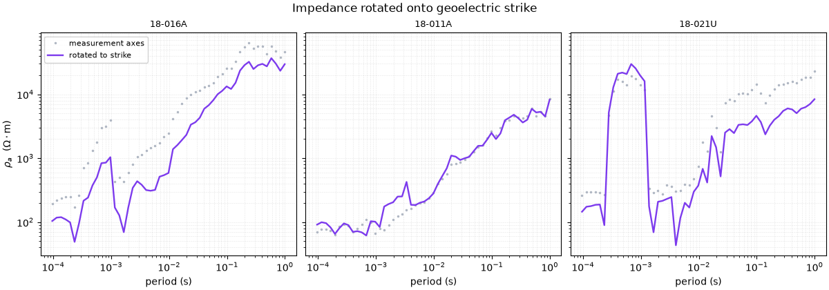
rotate_to_strike() rotates every station’s tensor so the off-diagonal (xy/yx) components carry the along/across-strike response. The xy apparent resistivity therefore changes — this is the data the 2-D solver actually inverts.

S_rot = rotate_to_strike(S, recursive=False)
rot = curves(S_rot, "rho")

stations = list(raw)
pick = [stations[3], stations[len(stations) // 2], stations[-4]]
plot_before_after(
    raw,
    rot,
    pick,
    quantity="rho",
    labels=("measurement axes", "rotated to strike"),
    colors=("#b0b7c3", "#7c3aed"),
    title="Impedance rotated onto geoelectric strike",
)

<Figure size 1200x420 with 3 Axes>

Does rotation improve 2-D-ness?

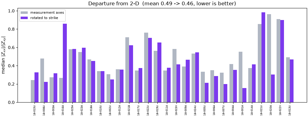
A 2-D tensor has strong off-diagonal and near-zero diagonal components. The ratio |Zxx| / |Zxy| measures the departure from that ideal; rotating to strike should push it down. We compare the median ratio per station, before and after.

def diag_ratio(sites):
    out = []
    for _i, ed in enumerate(_iter_items(sites)):
        z = np.asarray(ed.z if hasattr(ed, "z") else ed.Z.z)
        num = np.abs(z[:, 0, 0]) + np.abs(z[:, 1, 1])
        den = np.abs(z[:, 0, 1]) + np.abs(z[:, 1, 0]) + 1e-12
        out.append(np.nanmedian(num / den))
    return np.array(out)


r_before = diag_ratio(S)
r_after = diag_ratio(S_rot)
x = np.arange(len(r_before))
import matplotlib.pyplot as plt

fig, ax = plt.subplots(figsize=(10, 3.8), constrained_layout=True)
ax.bar(
    x - 0.2, r_before, width=0.4, color="#b0b7c3", label="measurement axes"
)
ax.bar(
    x + 0.2, r_after, width=0.4, color="#7c3aed", label="rotated to strike"
)
ax.set_xticks(x)
ax.set_xticklabels(stations, rotation=90, fontsize=6)
ax.set_ylabel(r"median $|Z_{xx}|/|Z_{xy}|$")
ax.set_title(
    f"Departure from 2-D  (mean {r_before.mean():.2f} -> "
    f"{r_after.mean():.2f}, lower is better)"
)
ax.legend(fontsize=8)

<matplotlib.legend.Legend object at 0x7f2a995e2030>

Antisymmetrise for 2-D inversion

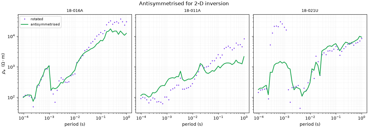
antisymmetrize() enforces Zxy = -Zyx exactly, projecting the tensor onto the ideal 2-D form — a common final step before handing data to a 2-D solver that expects it.

S_anti = antisymmetrize(S_rot, recursive=False)
anti = curves(S_anti, "rho")
plot_before_after(
    rot,
    anti,
    pick,
    quantity="rho",
    labels=("rotated", "antisymmetrised"),
    colors=("#7c3aed", "#16a34a"),
    title="Antisymmetrised for 2-D inversion",
)

/opt/build/repo/pycsamt/z/utils.py:396: ComplexWarning: Casting complex values to real discards the imaginary part
  E = ensure_z3(z_err).astype(float, copy=False)

<Figure size 1200x420 with 3 Axes>

Takeaway. Estimate the strike, confirm it is consistent along the line, rotate onto it, and (for a 2-D solver) antisymmetrise — the diagonal-ratio drop confirms the tensor is closer to the 2-D ideal. All four waves come together in the publication workflow.