
Note
Go to the end to download the full example code.
Processing a tipper survey (spectra to induction arrows)#
The corrections so far worked on the impedance tensor; this one follows the
vertical-field tipper through a complete run. MT data begins life as raw
cross-spectra, from which both the impedance and the tipper are derived —
so we open at the spectra level, then process a real tipper-bearing line
(KAP03, a SAMTEX long-period profile whose station coordinates live in
the hidden REFLAT/REFLONG fields), watching the induction response
clean up and writing tipper-preserving EDIs at the end.
Where tipper comes from: the raw spectra#
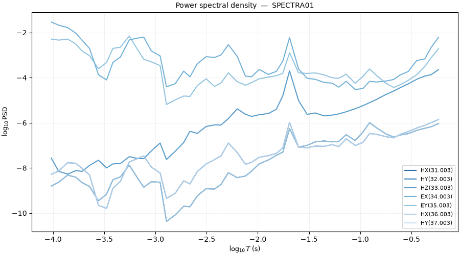
Spectra.from_file reads the
>=SPECTRASECT cross-power block. plot_psd()
shows the channel power spectra — the signal levels every transfer function
is estimated from.
import os
from pathlib import Path

import numpy as np

from pycsamt.emtools import (
    plot_psd,
    plot_tipper_from_spectra,
    spectra_summary,
)
from pycsamt.seg.spectra import Spectra

ROOT = Path(os.environ.get("PYCSAMT_DOCS_REPO_ROOT", "."))
sp = Spectra.from_file(str(ROOT / "data" / "MT" / "SPECTRA" / "spectra01.edi"))
print("spectra summary:")
print(spectra_summary(sp))
_ax = plot_psd(sp)
spectra summary:
APIFrame: spectra_summary
kind: emtools.spectra.summary
shape: 51 rows x 13 columns
columns: freq, period, bw, avgt, rotspec, psd_HX(31.003), psd_HY(32.003), psd_HZ(33.003), ...
numeric: 13 columns
missing: 0.0%
source: Spectra: SPECTRA01
n_freq: 51
f[Hz]: min=1.72, max=10400
errors: no
arrays:
  - _freq: (51,)@float64
  - _S: (51, 7, 7)@complex128
  - bw: (51,)@float64
  - avgt: (51,)@float64
  - avgf: (51,)@float64
  - rotspec: (51,)@float64
  - segnum: (51,)@int64
  - _S_fcu: (51, 7, 7)@complex128
  - _missing_mask: (51, 7, 7)@bool
  - avgt_present: (51,)@bool
  - rotspec_present: (51,)@bool
description: Compact per-frequency spectra summary.
The tipper, recovered from the spectra#
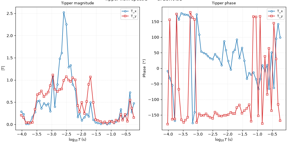
plot_tipper_from_spectra() solves the vertical-field
transfer function (Tx, Ty) straight from the cross-spectra — the tipper
at its origin, before it is written into an EDI. This is the quantity the
rest of the workflow conditions.
Load the tipper line#
KAP03 ships the derived impedance and tipper. Its 26 stations span 25 s - 17,067 s, and unlike the AMT lines it carries a genuine vertical field, so every induction arrow below is real tipper.
from pycsamt.emtools import (
    drop_duplicates,
    drop_low_confidence_frequencies,
    notch_powerline,
    plot_induction_arrows,
    plot_induction_rose,
    plot_induction_section,
    select_band,
    smooth_logfreq,
)
from pycsamt.emtools._core import _iter_items, ensure_sites
from pycsamt.site.export import write_sites

K = ensure_sites(str(ROOT / "data" / "MT" / "kap03lmt_edis"))


def n_freq(sites):
    return np.array([len(np.asarray(e.freq)) for e in _iter_items(sites)])


print(
    f"KAP03: {len(n_freq(K))} stations, {n_freq(K).max()} frequencies "
    f"(period 25-17067 s), real tipper channel"
)
KAP03: 26 stations, 20 frequencies (period 25-17067 s), real tipper channel
Raw induction arrows#
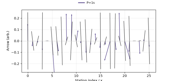
plot_induction_arrows() draws the real induction
vectors at several periods. Under the Parkinson convention they point
away from conductors, so a coherent arrow pattern is real structure and a
noisy one flags tipper that needs cleaning.
Raw tipper section#
plot_induction_section() images tipper magnitude
across station and period — effectively a spectral view of the vertical
field. The raw section is speckled where the tipper estimate is noisy.
ax = plot_induction_section(K, component="real")
![Tipper section [real]](../../_images/sphx_glr_plot_7_tipper_processing_004.png)
Process the survey (tipper carried through)#
The correction functions accept also="both", so they clean the
tipper alongside the impedance. We trim the frequency axis, then notch
and smooth — each step returning a new Sites whose tipper is processed,
not dropped.
s1 = drop_duplicates(K, recursive=False)
s2 = select_band(s1, fmin=1e-4, fmax=5e-2, recursive=False)
s3 = drop_low_confidence_frequencies(s2, threshold=0.5, recursive=False)
s4 = notch_powerline(s3, also="both", recursive=False)
final = smooth_logfreq(s4, win=5, also="both", recursive=False)
print(
    f"frequencies: {n_freq(K).max()} raw -> {n_freq(final).max()} processed "
    f"(band-trimmed and confidence-pruned)"
)
print(
    "chain: raw -> drop_dup -> select_band -> drop_low_conf -> "
    "notch(both) -> smooth(both)"
)
frequencies: 20 raw -> 18 processed (band-trimmed and confidence-pruned)
chain: raw -> drop_dup -> select_band -> drop_low_conf -> notch(both) -> smooth(both)
Processed tipper section#
The same section on the processed data: band-limited to the trustworthy periods and smoothed, so the coherent induction signal stands clear of the noise the raw section carried.
ax = plot_induction_section(final, component="real")
![Tipper section [real]](../../_images/sphx_glr_plot_7_tipper_processing_005.png)
Processed induction rose#
plot_induction_rose() folds the arrow azimuths into
a rose — after cleaning, a tighter preferred direction confirms a coherent
regional conductor rather than scatter.
ax = plot_induction_rose(final, component="real")
![Induction arrow rose [real]](../../_images/sphx_glr_plot_7_tipper_processing_006.png)
Write tipper-preserving EDIs#
write_sites() serialises the processed line back
to EDIs with the cleaned tipper intact — the deliverable for a
tipper-inclusive inversion.
import tempfile

outdir = Path(tempfile.mkdtemp(prefix="kap03_tipper_"))
paths = write_sites(final, outdir, exist_ok=True)
reloaded = ensure_sites(str(outdir))
print(
    f"wrote {len(paths)} tipper-preserving EDIs; re-loaded "
    f"{len(n_freq(reloaded))} with {n_freq(reloaded).max()} frequencies"
)
wrote 26 tipper-preserving EDIs; re-loaded 26 with 18 frequencies
Takeaway. Tipper rides through the same Sites -> Sites pipeline as
the impedance: process it with also="both", watch the induction section
and rose clean up, and write EDIs that keep the vertical field. Combined
with the impedance waves (static shift, rotation), this completes a
tipper-inclusive processing run — spectra in, sanitised induction arrows
out.
Total running time of the script: (0 minutes 1.629 seconds)