Groom-Bailey galvanic distortion (pycsamt.emtools.gb)

pycsamt.emtools.gb fits a real, frequency-independent 2x2 distortion matrix \(D\) so that \(Z_{obs}(f) \approx D\,Z_{2D}(f)\) for an anti-diagonal regional tensor \(Z_{2D}\), then decomposes \(D\) into gain, twist, shear, and anisotropy-style parameters. It is classic MT machinery (Groom & Bailey 1989), but nothing about the fit depends on the source being natural rather than controlled — the galvanic-distortion assumption (local, frequency-independent scattering of the electric field) applies identically to AMT, which is simply higher-frequency natural-source MT. This example therefore uses the same L18PLT (data/AMT/WILLY_DATA/) line as most of the other emtools examples, not a dedicated MT line.

Note

Section 6 below surfaces a genuine, verifiable property rather than a bug: applying the fitted correction changes every impedance-derived quantity, but leaves classify_dimensionality()’s frac_3d completely unchanged, station for station. That is not a null result — the phase tensor \(\Phi = \operatorname{Re}(Z)^{-1} \operatorname{Im}(Z)\) is mathematically invariant to any real, frequency-independent distortion matrix \(D\) (Caldwell, Bibby & Brown 2004), and classify_dimensionality is built entirely from phase-tensor features. Section 6 demonstrates this directly instead of only asserting it.

1. Fitting a distortion table without applying anything

groom_bailey_table() never mutates the survey; it only reports one fitted-parameter row per station.

import matplotlib.pyplot as plt
import numpy as np
import pandas as pd
from _datasets import load_survey

from pycsamt.emtools import (
    apply_groom_bailey,
    groom_bailey_decomposition,
    groom_bailey_table,
)
from pycsamt.emtools.dimensionality import pre2d_inversion_assessment

survey = load_survey("amt_l18plt")
BAND = (1e-3, 10.0)

table = groom_bailey_table(survey, band=BAND, robust=True)
print(table["status"].value_counts())
print(f"rms_fit: mean={table['rms_fit'].mean():.3f}  max={table['rms_fit'].max():.3f}")

fig, ax = plt.subplots(figsize=(6, 6))
improved = table["diagonal_ratio_after"] < table["diagonal_ratio_before"]
ax.scatter(
    table.loc[improved, "diagonal_ratio_before"],
    table.loc[improved, "diagonal_ratio_after"],
    color="#2ca02c",
    label="improved",
)
ax.scatter(
    table.loc[~improved, "diagonal_ratio_before"],
    table.loc[~improved, "diagonal_ratio_after"],
    color="#d62728",
    label="not improved",
)
lims = [0.0, table[["diagonal_ratio_before", "diagonal_ratio_after"]].values.max() * 1.05]
ax.plot(lims, lims, "--", color="0.5", lw=1, label="no change")
ax.set_xlim(lims)
ax.set_ylim(lims)
ax.set_xlabel("Diagonal ratio, before")
ax.set_ylabel("Diagonal ratio, after")
ax.set_aspect("equal")
ax.legend(fontsize=8)
ax.set_title("L18PLT — Groom-Bailey diagonal-ratio change, all 28 stations")

status
ok    28
Name: count, dtype: int64
rms_fit: mean=0.296  max=0.552

Text(0.5, 1.0, 'L18PLT — Groom-Bailey diagonal-ratio change, all 28 stations')

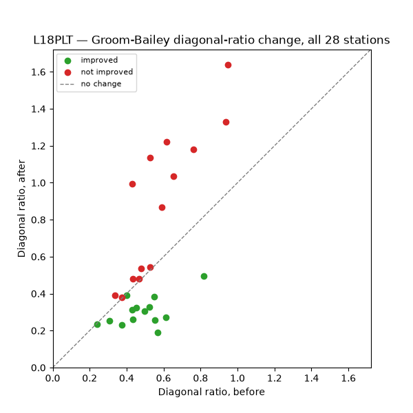
Reading this figure. Every one of the 28 stations has status == "ok" for this band. Points below the dashed \(y=x\) line got a lower diagonal ratio after fitting — 14 of 28 stations here, exactly half. The other half are not fit failures; they are stations where the frequency-independent-real-distortion model is a poor description of what is actually going on, which is exactly why groom_bailey_table reports diagnostics up front rather than silently “correcting” every station.

2. Which stations need the closest look

Sorting by rms_fit surfaces the stations least well described by the fitted model — the ones to inspect before trusting a blanket correction.

ranked = table.sort_values("rms_fit", ascending=False)

fig, ax = plt.subplots(figsize=(7, 6))
colors = ["#d62728" if v >= 0.25 else "#1f77b4" for v in ranked["rms_fit"].head(10)]
ax.barh(ranked["station"].head(10), ranked["rms_fit"].head(10), color=colors)
ax.axvline(0.25, color="0.3", ls="--", lw=1, label="rms_fit = 0.25")
ax.invert_yaxis()
ax.set_xlabel("rms_fit")
ax.legend(fontsize=8)
ax.set_title("L18PLT — 10 worst Groom-Bailey fits")
fig.tight_layout()

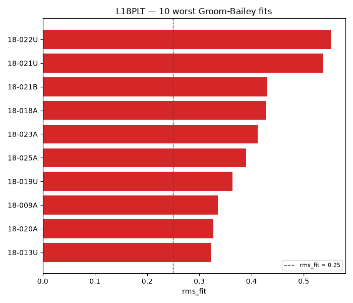
Reading this figure. 18-022U has the single highest residual, but the whole top-10 sits above rms_fit = 0.25 — the same threshold used below to decide which stations are safe to correct automatically, and a reminder that only a minority of this line’s 28 stations end up accepted.

3. Strike rotation changes the twist estimate, not just the fit

rotate_deg rotates the tensor before fitting. Comparing an unrotated fit against one rotated toward a plausible line strike shows how much of the “twist” GB reports is really just axis misalignment.

norot = groom_bailey_table(survey, band=BAND, robust=True, rotate_deg=None)
rot35 = groom_bailey_table(survey, band=BAND, robust=True, rotate_deg=35.0)
cmp_rot = norot[["station", "twist_deg", "rms_fit"]].merge(
    rot35[["station", "twist_deg", "rms_fit"]],
    on="station",
    suffixes=("_norot", "_rot35"),
)

fig, ax = plt.subplots(figsize=(6, 6))
ax.scatter(cmp_rot["twist_deg_norot"], cmp_rot["twist_deg_rot35"], color="#1f77b4")
lims = [
    min(cmp_rot["twist_deg_norot"].min(), cmp_rot["twist_deg_rot35"].min()) - 2,
    max(cmp_rot["twist_deg_norot"].max(), cmp_rot["twist_deg_rot35"].max()) + 2,
]
ax.plot(lims, lims, "--", color="0.5", lw=1)
ax.axhline(0, color="0.85", lw=0.8)
ax.axvline(0, color="0.85", lw=0.8)
ax.set_xlim(lims)
ax.set_ylim(lims)
ax.set_xlabel(r"twist$_{\deg}$, no rotation")
ax.set_ylabel(r"twist$_{\deg}$, rotated 35°")
ax.set_aspect("equal")
ax.set_title("L18PLT — twist before vs. after a 35° strike rotation")

print(
    f"mean |twist|: no rotation={cmp_rot['twist_deg_norot'].abs().mean():.1f} deg, "
    f"rotated 35 deg={cmp_rot['twist_deg_rot35'].abs().mean():.1f} deg"
)
print(
    f"mean rms_fit: no rotation={cmp_rot['rms_fit_norot'].mean():.3f}, "
    f"rotated 35 deg={cmp_rot['rms_fit_rot35'].mean():.3f}"
)

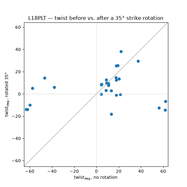
mean |twist|: no rotation=28.1 deg, rotated 35 deg=12.1 deg
mean rms_fit: no rotation=0.296, rotated 35 deg=0.323

Reading this figure/output. Rotating toward 35° roughly halves the mean absolute twist across the line (28.1° to 12.1°) — consistent with 35° being closer to this line’s true regional strike than the raw acquisition axes. But mean rms_fit gets slightly worse (0.296 to 0.323), not better: a single strike angle does not fit every station equally well along a real line, and several points sit far off the diagonal here. This is exactly why the page this example accompanies warns against picking rotate_deg to minimize the GB residual — strike should come from the strike/dimensionality workflow, and GB applied afterward, not the other way around.

4. Robust vs. non-robust weighting

With robust=True, later iterations downweight high-residual frequencies with a Huber-style rule instead of fitting them at full weight.

robust = groom_bailey_table(survey, band=BAND, robust=True, api=False)
plain = groom_bailey_table(survey, band=BAND, robust=False, api=False)
cmp_rw = robust.merge(plain, on="station", suffixes=("_robust", "_plain"))
cmp_rw["twist_diff"] = (cmp_rw["twist_deg_robust"] - cmp_rw["twist_deg_plain"]).abs()

fig, ax = plt.subplots(figsize=(6, 6))
ax.scatter(cmp_rw["twist_deg_plain"], cmp_rw["twist_deg_robust"], color="#9467bd")
lims = [
    min(cmp_rw["twist_deg_plain"].min(), cmp_rw["twist_deg_robust"].min()) - 2,
    max(cmp_rw["twist_deg_plain"].max(), cmp_rw["twist_deg_robust"].max()) + 2,
]
ax.plot(lims, lims, "--", color="0.5", lw=1)
ax.set_xlim(lims)
ax.set_ylim(lims)
ax.set_xlabel(r"twist$_{\deg}$, robust=False")
ax.set_ylabel(r"twist$_{\deg}$, robust=True")
ax.set_aspect("equal")
worst = cmp_rw.loc[cmp_rw["twist_diff"].idxmax()]
ax.annotate(
    worst["station"],
    (worst["twist_deg_plain"], worst["twist_deg_robust"]),
    textcoords="offset points",
    xytext=(6, 6),
    fontsize=8,
)
ax.set_title("L18PLT — robust vs. plain twist estimate")

print(f"mean |twist_robust - twist_plain|: {cmp_rw['twist_diff'].mean():.1f} deg")
print(f"largest divergence: {worst['station']} ({worst['twist_diff']:.1f} deg)")

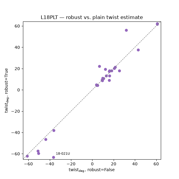
mean |twist_robust - twist_plain|: 4.5 deg
largest divergence: 18-021U (26.7 deg)

Reading this figure/output. Most stations sit close to the diagonal — robust weighting is a mild correction here, not a wholesale change. One station, 18-021U, diverges by nearly 27° between the two modes, a useful flag that its frequency band likely has one or more outlier rows distorting the plain (unweighted) fit.

5. Applying correction to accepted stations only

Filtering by fit quality before calling apply_groom_bailey() keeps a blanket correction from being applied to stations the fit does not actually support.

accepted = table.loc[
    (table["status"] == "ok")
    & (table["rms_fit"] < 0.25)
    & (table["diagonal_ratio_after"] < table["diagonal_ratio_before"])
].copy()
print(f"accepted: {len(accepted)} of {len(table)} stations")

corrected = apply_groom_bailey(survey, table=accepted, inplace=False)

fig, ax = plt.subplots(figsize=(7, 4.5))
x = np.arange(len(accepted))
width = 0.35
ax.bar(x - width / 2, accepted["diagonal_ratio_before"], width, label="before", color="#7f7f7f")
ax.bar(x + width / 2, accepted["diagonal_ratio_after"], width, label="after", color="#2ca02c")
ax.set_xticks(x)
ax.set_xticklabels(accepted["station"], rotation=45, ha="right", fontsize=8)
ax.set_ylabel("Diagonal ratio")
ax.legend(fontsize=8)
ax.set_title("L18PLT — diagonal ratio for the 6 accepted stations")
fig.tight_layout()

mean_before = accepted["diagonal_ratio_before"].mean()
mean_after = accepted["diagonal_ratio_after"].mean()
print(
    f"mean diagonal ratio: {mean_before:.3f} -> {mean_after:.3f} "
    f"({100 * (1 - mean_after / mean_before):.0f}% reduction)"
)

accepted: 6 of 28 stations
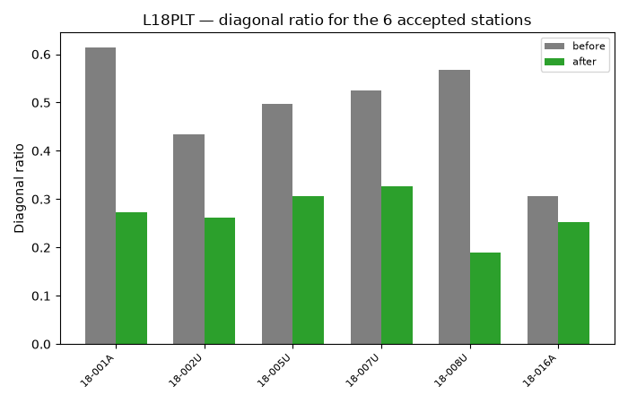
mean diagonal ratio: 0.491 -> 0.268 (45% reduction)

Reading this figure/output. All 6 accepted stations improve, by construction (that was the acceptance rule), but the improvement is real and substantial: diagonal ratio drops by 45% on average across the accepted subset. This is the payoff for filtering first rather than correcting every station the table happens to return.

6. Advanced: correction changes Z, but not the phase tensor

pre2d_inversion_assessment() reports frac_3d from phase-tensor features (classify_dimensionality()). Running it on both the GB-corrected sites and the untouched sites tests directly whether the correction changes that number.

gb_on = groom_bailey_decomposition(survey, apply=True, band=BAND, robust=True)
gb_off = groom_bailey_decomposition(survey, apply=False, band=BAND, robust=True)

assess_on = pre2d_inversion_assessment(
    gb_on.sites, band=BAND, groom_bailey_attempted=True, groom_bailey_applied=True
)
assess_off = pre2d_inversion_assessment(
    gb_off.sites, band=BAND, groom_bailey_attempted=True, groom_bailey_applied=False
)
cmp_dim = assess_on[["station", "frac_3d"]].merge(
    assess_off[["station", "frac_3d"]], on="station", suffixes=("_corrected", "_raw")
)
max_delta = (cmp_dim["frac_3d_corrected"] - cmp_dim["frac_3d_raw"]).abs().max()
print(f"max |frac_3d_corrected - frac_3d_raw| across all stations: {max_delta:.10f}")

fig, ax = plt.subplots(figsize=(5, 5))
ax.scatter(cmp_dim["frac_3d_raw"], cmp_dim["frac_3d_corrected"], color="#1f77b4")
ax.plot([0, 1], [0, 1], "--", color="0.5", lw=1)
ax.set_xlim(0, 1)
ax.set_ylim(0, 1)
ax.set_aspect("equal")
ax.set_xlabel("frac_3d, uncorrected")
ax.set_ylabel("frac_3d, GB-corrected")
ax.set_title("L18PLT — dimensionality is distortion-invariant")

max |frac_3d_corrected - frac_3d_raw| across all stations: 0.0000000000

Text(0.5, 1.0, 'L18PLT — dimensionality is distortion-invariant')

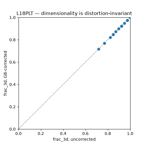
Reading this figure/output. Every point sits exactly on the \(y=x\) line; the maximum difference across all 28 stations is 0.0 to machine precision. That is the phase tensor’s defining property, not a limitation of this implementation: because \(\Phi = \operatorname{Re}(Z)^{-1}\operatorname{Im}(Z)\) and \(Z_{obs} = D\,Z_{2D}\) for a real matrix \(D\), the \(D\) cancels out of \(\Phi\) exactly. Any diagnostic built on phase-tensor skew and ellipticity — including this survey’s dimensionality classification — is blind to galvanic distortion by construction. Practically: running Groom-Bailey before a pre2d_inversion_assessment changes nothing about that assessment; it matters for the impedance-based quantities (apparent resistivity, static-shift-sensitive amplitudes) that GB actually corrects.

7. Synthetic sanity check

A small hand-built distorted 2-D tensor gives a known-answer check: with no noise, the fit should recover a near-zero residual and collapse the diagonal leakage to (numerical) zero.

class ZBlock:
    def __init__(self, z, freq):
        self.z = z
        self.freq = freq
        self.z_err = None


class Site:
    station = "SYN001"

    def __init__(self, z, freq):
        self.Z = ZBlock(z, freq)


freq_syn = np.logspace(0, 3, 12)
regional = np.zeros((freq_syn.size, 2, 2), dtype=complex)
regional[:, 0, 1] = 1.0 + 0.2j
regional[:, 1, 0] = -0.8 + 0.1j
D_true = np.array([[1.0, 0.25], [-0.15, 1.1]])
observed = D_true[None, :, :] @ regional
syn_table = groom_bailey_table([Site(observed, freq_syn)], robust=False)
print(
    syn_table[
        ["station", "rms_fit", "diagonal_ratio_before", "diagonal_ratio_after"]
    ].to_string(index=False)
)

station      rms_fit  diagonal_ratio_before  diagonal_ratio_after
 SYN001 3.678917e-16               0.187225          4.388355e-17

Reading this output. rms_fit lands at machine precision (~1e-16) and the diagonal ratio collapses from 0.19 to ~4e-17 — exactly what a noise-free synthetic distortion should produce, and a useful regression check whenever the fitting code changes.