
Note
Go to the end to download the full example code.
Galvanic-distortion case study with Groom–Bailey correction#
Static shift moves apparent-resistivity curves up or down. Tensor rotation changes the coordinate frame. A deeper correction question is:
does the impedance tensor carry a frequency-independent galvanic distortion matrix that should be estimated and removed before 2-D interpretation?
This example builds that decision as a case study. We estimate a Groom–Bailey-style real distortion matrix per station, audit the fitted parameters, apply the correction, and then compare the original and corrected responses. The goal is not to blindly make the curves prettier. The goal is to decide whether the correction is physically plausible, stable across the line, and limited to the tensor distortion it is meant to remove.
1. Imports and data#
The example uses public pycsamt.emtools functions for the actual
correction and the small gallery helper only for loading the bundled WILLY
line and extracting curves for plotting.
import os
import sys
from pathlib import Path

import matplotlib.pyplot as plt
import numpy as np


def repo_root():
    root = os.environ.get("PYCSAMT_DOCS_REPO_ROOT")
    return Path(root) if root else Path(__file__).resolve().parents[3]


ROOT = repo_root()
if str(ROOT) not in sys.path:
    sys.path.insert(0, str(ROOT))

from _corr_data import curves, demo_line, plot_before_after

from pycsamt.emtools import (
    apply_groom_bailey,
    groom_bailey_decomposition,
)
from pycsamt.emtools._core import _iter_items

S = demo_line("L18PLT")
raw_rho_xy = curves(S, quantity="rho", component="xy")
raw_rho_yx = curves(S, quantity="rho", component="yx")
stations = list(raw_rho_xy)
2. Choose a fitting band#
Groom–Bailey decomposition assumes a real, frequency-independent distortion matrix multiplying a simpler regional tensor. That assumption is more defensible over a controlled period band than over every available sample. Here we keep the AMT band used by the other correction examples, avoiding the shortest-period edge where local noise and instrument effects can dominate.
fit_band = (1e-4, 1.0)  # period seconds
gb = groom_bailey_decomposition(
    S,
    band=fit_band,
    apply=False,
    min_freq=8,
    robust=True,
    recursive=False,
)
table = gb.table
ok = table[table["status"] == "ok"].copy()

print(gb.summary())
print(f"Fit band: {fit_band[0]:.0e}-{fit_band[1]:.1f} s")
print(f"Stations fitted: {len(ok)} / {len(table)}")
print(
    "Median fit RMS: "
    f"{np.nanmedian(ok['rms_fit']):.3f}; "
    "median |twist|: "
    f"{np.nanmedian(np.abs(ok['twist_deg'])):.1f} deg"
)
GroomBaileyResult(stations=28, applied=False, median_rms=0.2391)
Fit band: 1e-04-1.0 s
Stations fitted: 28 / 28
Median fit RMS: 0.239; median |twist|: 13.1 deg
3. Audit the distortion parameters before applying them#
The table is the most important product of the fitting step. Large isolated twist, shear, anisotropy, or RMS values should be investigated before the correction is accepted. In production you may reject those stations, change the period band, rotate to strike first, or compare with phase-tensor diagnostics.
cols = [
    "station",
    "n_freq",
    "twist_deg",
    "shear",
    "anisotropy",
    "rms_fit",
    "diagonal_ratio_before",
]
print(ok[cols].head(8).to_string(index=False))

x = np.arange(len(ok))
station_labels = ok["station"].to_numpy()

fig, axs = plt.subplots(4, 1, figsize=(11.5, 8.8), sharex=True)

axs[0].bar(x, ok["twist_deg"], color="#2563eb")
axs[0].axhline(0.0, color="black", lw=0.8)
axs[0].set_ylabel("Twist (deg)")
axs[0].set_title("Groom--Bailey distortion audit before correction")

axs[1].bar(x - 0.18, ok["shear"], width=0.36, color="#7c3aed", label="shear")
axs[1].bar(
    x + 0.18,
    ok["anisotropy"],
    width=0.36,
    color="#0891b2",
    label="anisotropy",
)
axs[1].axhline(0.0, color="black", lw=0.8)
axs[1].set_ylabel("Parameter")
axs[1].legend(fontsize=8, ncol=2)

axs[2].bar(x, ok["rms_fit"], color="#f97316")
axs[2].axhline(np.nanmedian(ok["rms_fit"]), color="black", lw=1.0, ls="--")
axs[2].set_ylabel("RMS fit")

axs[3].bar(x, ok["diagonal_ratio_before"], color="#64748b")
axs[3].set_ylabel("diag/offdiag")
axs[3].set_xlabel("Station")
axs[3].set_xticks(x)
axs[3].set_xticklabels(station_labels, rotation=90, fontsize=7)

for ax in axs:
    ax.grid(axis="y", alpha=0.25)

fig.tight_layout()
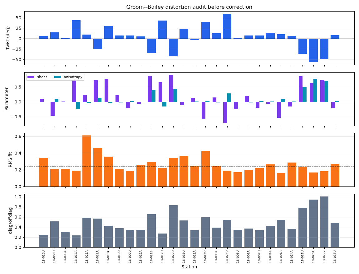
station  n_freq  twist_deg     shear  anisotropy  rms_fit  diagonal_ratio_before
18-001A      52  10.102875 -0.528220    0.082754 0.158575               0.544145
18-002U      52   7.300827 -0.215363    0.019708 0.184191               0.347040
18-003A      52   0.561317  0.010808   -0.000017 0.213355               0.303098
18-004A      52  13.649939 -0.063763    0.014045 0.263806               0.421946
18-005U      52   1.548812 -0.248284    0.004819 0.170825               0.347734
18-006A      52   7.101233  0.199993   -0.019971 0.202384               0.372353
18-007U      52   7.082999 -0.202458    0.016803 0.218972               0.341553
18-008U      52  14.410432 -0.473655    0.081644 0.207660               0.514751
4. Inspect the fitted distortion matrices#
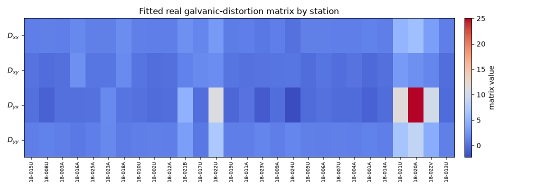
Each station has a 2x2 real matrix D. The heat maps below are a compact
way to see whether the line behaves coherently. A smooth survey-scale
pattern is easier to defend than a correction driven by one wild station.
matrix_fields = [
    "distortion_xx",
    "distortion_xy",
    "distortion_yx",
    "distortion_yy",
]
matrix_panel = ok[matrix_fields].to_numpy(dtype=float).T

fig, ax = plt.subplots(figsize=(11.0, 3.8))
im = ax.imshow(matrix_panel, aspect="auto", cmap="coolwarm")
ax.set_yticks(np.arange(4))
ax.set_yticklabels([r"$D_{xx}$", r"$D_{xy}$", r"$D_{yx}$", r"$D_{yy}$"])
ax.set_xticks(x)
ax.set_xticklabels(station_labels, rotation=90, fontsize=7)
ax.set_title("Fitted real galvanic-distortion matrix by station")
cbar = fig.colorbar(im, ax=ax, pad=0.02)
cbar.set_label("matrix value")
fig.tight_layout()
5. Apply the correction after the audit#
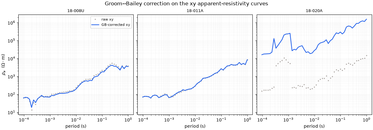
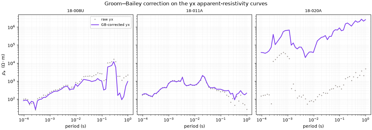
apply_groom_bailey removes the fitted matrix from each station:
Z_corrected = inv(D) @ Z_observed.
The correction is applied to a copy because gallery examples should not
mutate the original dataset. If you want one object that bundles the table
and the corrected sites, call groom_bailey_decomposition(..., apply=True).
S_gb = apply_groom_bailey(S, table=table, recursive=False, inplace=False)
corr_rho_xy = curves(S_gb, quantity="rho", component="xy")
corr_rho_yx = curves(S_gb, quantity="rho", component="yx")

pick = [
    station_labels[1],
    station_labels[len(station_labels) // 2],
    station_labels[-3],
]

plot_before_after(
    raw_rho_xy,
    corr_rho_xy,
    pick,
    quantity="rho",
    labels=("raw xy", "GB-corrected xy"),
    colors=("#a8a29e", "#2563eb"),
    title="Groom--Bailey correction on the xy apparent-resistivity curves",
)

plot_before_after(
    raw_rho_yx,
    corr_rho_yx,
    pick,
    quantity="rho",
    labels=("raw yx", "GB-corrected yx"),
    colors=("#a8a29e", "#7c3aed"),
    title="Groom--Bailey correction on the yx apparent-resistivity curves",
)
<Figure size 1200x420 with 3 Axes>
6. Quantify what changed#
A correction should have a measurable footprint, but not an uncontrolled one. We summarize the median change in log10 apparent resistivity for each station and compare the tensor diagonal/off-diagonal ratio before and after.
def tensor_diag_ratio(sites):
    out = []
    for ed in _iter_items(sites):
        z = np.asarray(ed.z if hasattr(ed, "z") else ed.Z.z)
        diag = np.sqrt(np.abs(z[:, 0, 0]) ** 2 + np.abs(z[:, 1, 1]) ** 2)
        off = np.sqrt(np.abs(z[:, 0, 1]) ** 2 + np.abs(z[:, 1, 0]) ** 2)
        out.append(np.nanmedian(diag / np.maximum(off, 1e-24)))
    return np.asarray(out, dtype=float)


def station_log_change(before, after):
    changes = []
    for st in station_labels:
        _pb, vb = before[st]
        _pa, va = after[st]
        mask = np.isfinite(vb) & np.isfinite(va) & (vb > 0.0) & (va > 0.0)
        changes.append(np.nanmedian(np.log10(va[mask]) - np.log10(vb[mask])))
    return np.asarray(changes, dtype=float)


delta_xy = station_log_change(raw_rho_xy, corr_rho_xy)
delta_yx = station_log_change(raw_rho_yx, corr_rho_yx)
ratio_before = tensor_diag_ratio(S)
ratio_after = tensor_diag_ratio(S_gb)

fig, axs = plt.subplots(2, 1, figsize=(11.5, 6.5), sharex=True)

axs[0].bar(x - 0.18, delta_xy, width=0.36, color="#2563eb", label="xy")
axs[0].bar(x + 0.18, delta_yx, width=0.36, color="#7c3aed", label="yx")
axs[0].axhline(0.0, color="black", lw=0.8)
axs[0].set_ylabel(r"median $\Delta \log_{10}\rho_a$")
axs[0].set_title("Correction footprint by station")
axs[0].legend(fontsize=8, ncol=2)

axs[1].plot(x, ratio_before, "o-", color="#a8a29e", label="before")
axs[1].plot(x, ratio_after, "o-", color="#16a34a", label="after")
axs[1].set_ylabel("diag/offdiag")
axs[1].set_xlabel("Station")
axs[1].set_xticks(x)
axs[1].set_xticklabels(station_labels, rotation=90, fontsize=7)
axs[1].legend(fontsize=8)

for ax in axs:
    ax.grid(alpha=0.25)

fig.tight_layout()

print(
    "Median absolute correction: "
    f"xy={np.nanmedian(np.abs(delta_xy)):.3f} log10 units, "
    f"yx={np.nanmedian(np.abs(delta_yx)):.3f} log10 units"
)
print(
    "Median diagonal/off-diagonal ratio: "
    f"{np.nanmedian(ratio_before):.3f} -> {np.nanmedian(ratio_after):.3f}"
)
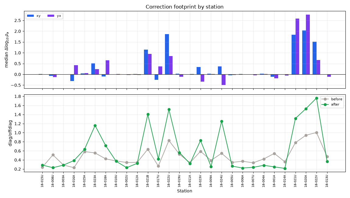
Median absolute correction: xy=0.045 log10 units, yx=0.111 log10 units
Median diagonal/off-diagonal ratio: 0.423 -> 0.369
7. Decision guide#
Use Groom–Bailey correction when the distortion parameters are stable enough to defend geologically and the fit is good in the selected band. Treat it as a diagnostic when:
one or two stations dominate the correction;
the fitted twist/shear changes sign erratically from station to station;
the correction improves one tensor component but damages another;
phase-tensor or strike diagnostics indicate strong 3-D structure.
The safest production workflow is:
run ordinary QC and remove bad frequencies;
estimate strike and dimensionality;
fit Groom–Bailey parameters over a defensible period band;
inspect the table and matrix heat map;
apply the correction only if the diagnostics support it.
Total running time of the script: (0 minutes 2.407 seconds)