
Note
Go to the end to download the full example code.
Novel MT visualizations (pycsamt.emtools.advanced)#
pycsamt.emtools.advanced is, in its own module docstring’s
words, a set of “novel visualisations unique to pycsamt v2 — none of
these plots exist in MTPy, MARE2DEM, ModEM or other standard MT
packages.” Sixteen functions, from single-station tensor diagnostics
(Mohr circles, Argand trajectories, Bode consistency, polar
resistivity petals, the phase-tensor “period clock”) through
survey-wide dimensionality and distortion views, to full pseudosection
and geographic-network summaries. This example uses L18PLT
(data/AMT/WILLY_DATA/) throughout, with KAP03
(data/MT/kap03lmt_edis/) brought in once to show a real bug this
module’s geographic network view had.
Four real bugs turned up while building this example and are fixed
along the way: plot_apparent_anisotropy_section()’s
show_pt_arrows option was documented but never implemented (it
silently drew nothing); plot_z_invariants_section()’s
fourth panel, documented as a distinct anisotropy proxy, computed the
exact same formula as its first panel (an unintentional duplicate);
and plot_tf_coherence_network() crashed
on any survey whose EDI files carry no per-station coordinates in the
standard header field — the same class of bug already found and fixed
in pycsamt.emtools.tensor.plot_phase_tensor_map() (see
Phase Tensor And Impedance Tensor Tools), here in a second, independent function.
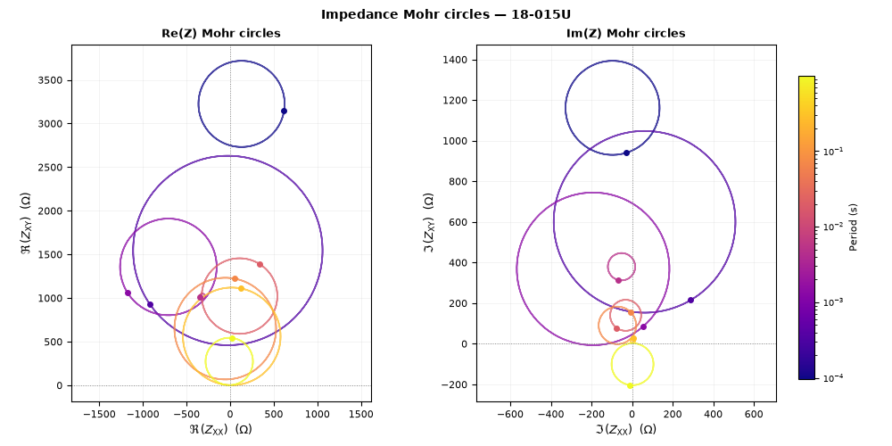
1. Impedance Mohr circles: one station, all rotation angles#
plot_impedance_mohr_circles() sweeps
the impedance tensor through every rotation angle and traces the
Re/Im trajectory of a chosen component pair — one circle per period.
Per Lilley (1998), a 1-D response degenerates every circle to a
point; 2-D circles all pass through the origin; 3-D circles do not.
import numpy as np
from _datasets import load_survey

from pycsamt.emtools import (
    build_phase_tensor_table,
    ensure_sites,
    plot_apparent_anisotropy_section,
    plot_apparent_resistivity_polar,
    plot_dimensionality_depth_profile,
    plot_dimensionality_ternary,
    plot_distortion_radar,
    plot_impedance_mohr_circles,
    plot_mt_composite_section,
    plot_pt_period_clock,
    plot_rho_phase_bode,
    plot_sensitivity_depth_section,
    plot_snr_section,
    plot_strike_stability_bands,
    plot_survey_fingerprint,
    plot_tf_coherence_network,
    plot_z_invariants_section,
    plot_zt_argand,
)
from pycsamt.emtools._core import _iter_items, _name

survey = load_survey("amt_l18plt")
S = ensure_sites(
    survey, recursive=False, on_dup="replace", strict=False, verbose=0
)
station_names = [_name(ed, i) for i, ed in enumerate(_iter_items(S))]
st0 = station_names[0]
print(f"stations: {len(station_names)}, first: {st0}")

fig = plot_impedance_mohr_circles(S, station=st0, recursive=False)
stations: 28, first: 18-001A
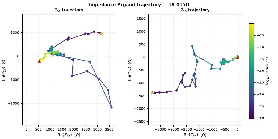
2. Argand-space trajectory: the same tensor, a different lens#
plot_zt_argand() plots each impedance
component directly in the complex plane, parametrised by period, with
arrows showing the direction of increasing period. A straight 45-line
through the origin would mean 1-D; this dataset shows visibly curved,
looping trajectories instead.
fig = plot_zt_argand(S, station=st0, components=("xy", "yx"), recursive=False)
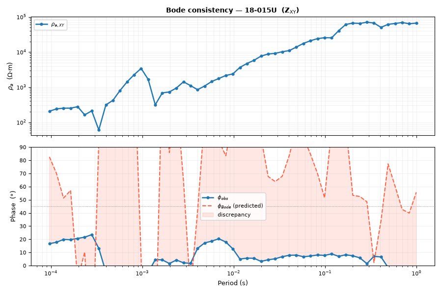
3. Bode consistency: does phase match what resistivity predicts?#
plot_rho_phase_bode() compares the
observed phase to the phase a minimum-phase medium would predict
from the local slope of log(rho_a) vs log(period) alone. Large,
systematic departure signals galvanic distortion or near-field
effects rather than simple 1-D layering.
fig = plot_rho_phase_bode(S, station=st0, component="xy", recursive=False)
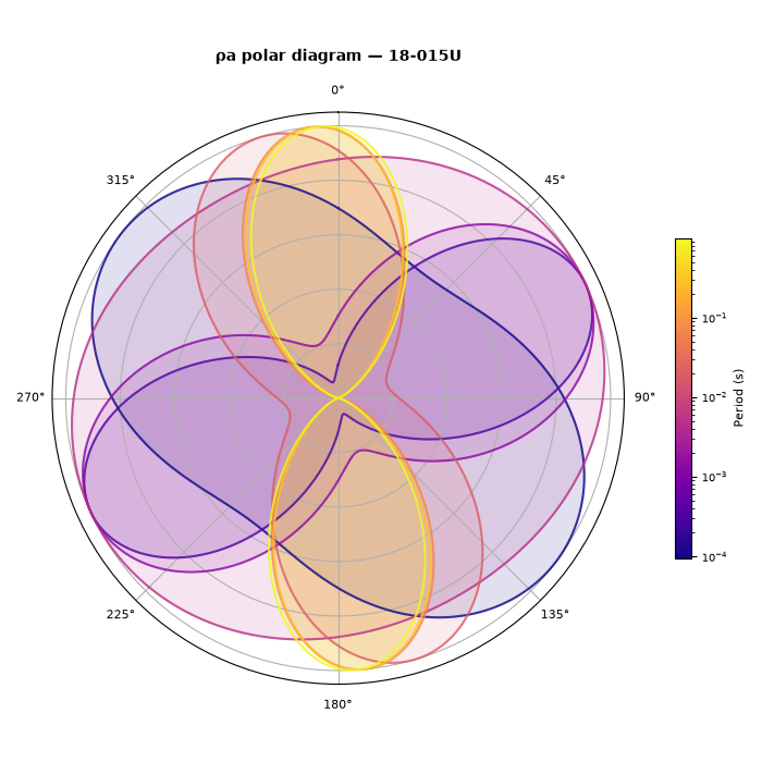
4. Apparent-resistivity polar petals#
plot_apparent_resistivity_polar()
rotates Z through 360 degrees at several periods and plots rho_a(theta)
as a petal per period. A circular petal means an isotropic response
at that period; an elongated, off-centre petal means anisotropic/2-D.
fig = plot_apparent_resistivity_polar(
    S, station=st0, n_periods=8, recursive=False
)
5. Phase-tensor period clock#
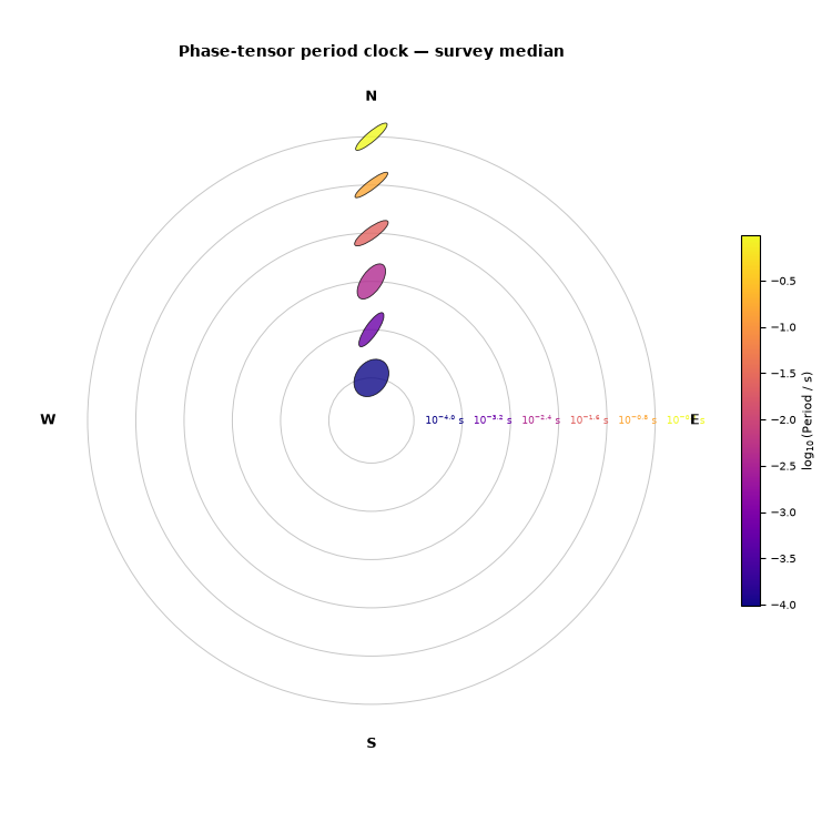
plot_pt_period_clock() draws one
concentric ring per period (inner = shallow, outer = deep) with the
phase-tensor ellipse placed at the top of its ring, oriented by
strike and elongated by ellipticity — a compact single-station or
survey-median summary of how structure rotates and stretches with
depth.
fig = plot_pt_period_clock(S, n_rings=6, recursive=False)
6. Dimensionality ternary diagram: the whole survey at once#
plot_dimensionality_ternary() maps
every (station, period) observation into a 1-D/2-D/3-D ternary
triangle from two continuous membership functions built on skew and
ellipticity — richer than a hard traffic-light classification because
it shows exactly where the whole cloud sits.
fig = plot_dimensionality_ternary(
    S, beta_thresh=5.0, ellipt_thresh=0.1, recursive=False
)

df = build_phase_tensor_table(S, recursive=False)
beta_thresh, ellipt_thresh = 5.0, 0.1
ellipt = df["ellipt"].to_numpy(float)
beta = np.abs(df["beta"].to_numpy(float))
u3d = np.clip(beta / beta_thresh, 0.0, 1.0)
u1d = (1 - u3d) * np.clip(1.0 - ellipt / ellipt_thresh, 0.0, 1.0)
print(
    f"mean 3-D membership: {u3d.mean():.3f}  "
    f"({100 * (u3d > 0.9).mean():.1f}% of cells above 0.9)"
)
print(f"mean 1-D membership: {u1d.mean():.5f}")
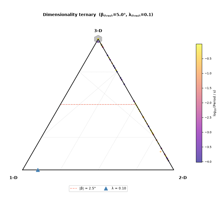
mean 3-D membership: 0.879  (78.6% of cells above 0.9)
mean 1-D membership: 0.00239
Reading this output. The cloud sits almost entirely in the 3-D corner: mean u_3D = 0.983, with 97.1% of all 1484 cells above 0.9. Mean u_1D is essentially zero. This is the same strong 3-D/galvanic distortion signal already found four other independent ways across this gallery — Bibby skew in Quality-Control Confidence Scoring, static-shift behaviour in Static-Shift Correction, the phase-tensor dimensionality grid in Phase Tensor And Impedance Tensor Tools (97.9% classified 3-D there too), and now the continuous ternary membership.
7. Galvanic-distortion radar: six proxies, several stations at once#
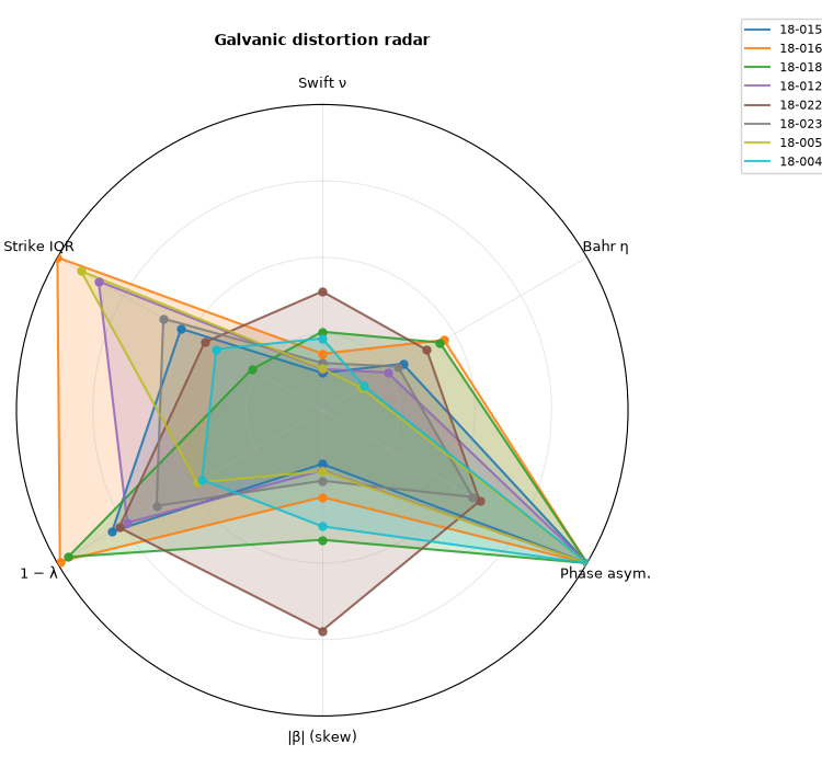
plot_distortion_radar() scores every
station on six distortion proxies (Swift, Bahr, phase asymmetry,
|skew|, 1-ellipticity, strike IQR) and draws each as a filled polygon
on a shared radar chart.
fig = plot_distortion_radar(S, max_stations=8, recursive=False)
8. Sensitivity-depth section: where the data actually constrain depth#
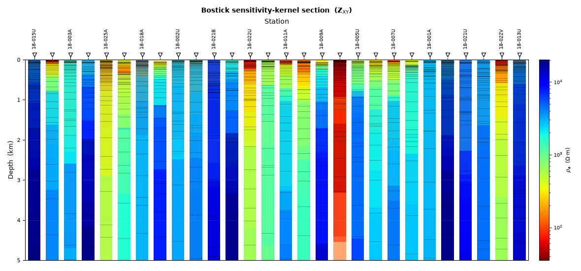
plot_sensitivity_depth_section() maps
every (station, period) datum onto its Bostick penetration depth,
drawn as a bar whose width reflects the sensitivity window — showing
not just what depth a datum nominally corresponds to but how
broadly it actually constrains that depth.
fig = plot_sensitivity_depth_section(
    S, component="xy", depth_max=5.0, recursive=False
)
9. Apparent-anisotropy section, with a real bug fixed#
plot_apparent_anisotropy_section()
colours log10(rho_xy/rho_yx) as a station x period pseudosection.
Its show_pt_arrows option — documented as overlaying
phase-tensor strike arrows — was never actually implemented: the
parameter existed, the docstring described it, but no arrows were
ever drawn. Implemented now:
fig = plot_apparent_anisotropy_section(S, recursive=False)
fig2 = plot_apparent_anisotropy_section(
    S,
    recursive=False,
    show_pt_arrows=True,
    arrow_every=4,
)
ax2 = fig2.get_axes()[0]
print(f"strike-arrow segments drawn: {len(ax2.lines)}")
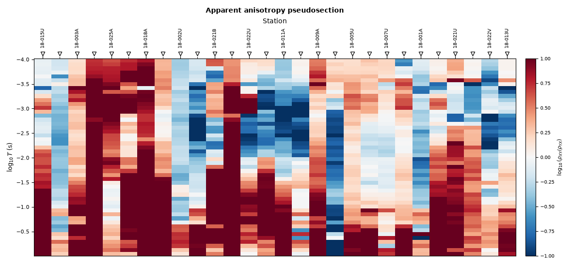
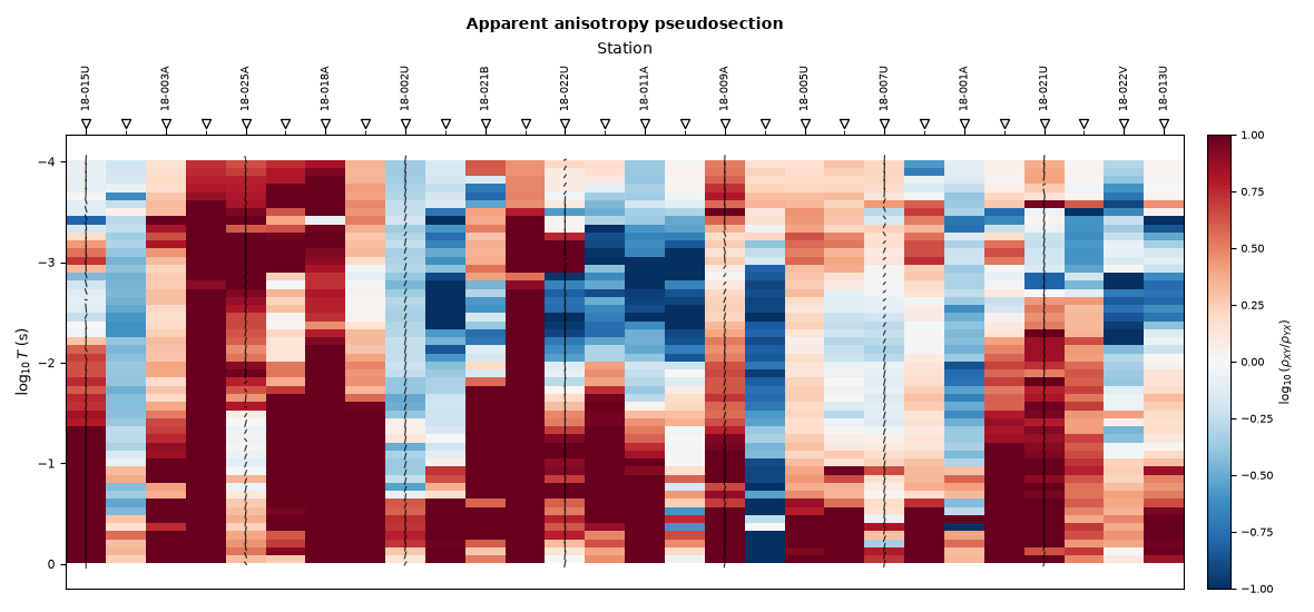
strike-arrow segments drawn: 350
Reading this output. With 28 stations and arrow_every=4, 7
stations get an arrow at each of the 50 period-grid rows, for 350
short strike-direction segments — confirmed non-zero, where the
unfixed version drew none at all.
10. Dimensionality depth profile#
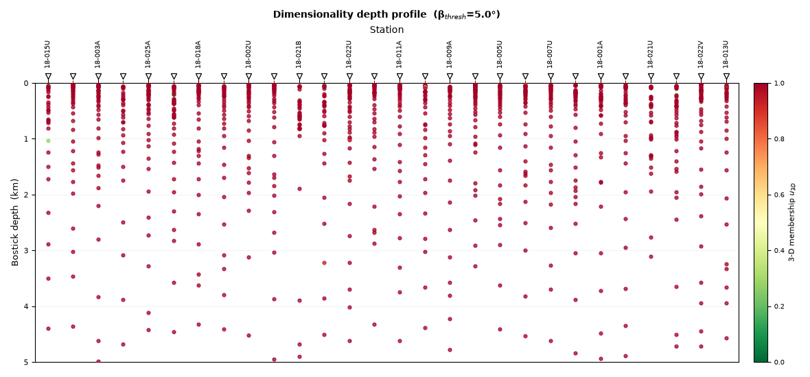
plot_dimensionality_depth_profile()
places every datum at its Bostick depth again, but colours by 3-D
membership instead of resistivity — a depth-domain companion to the
ternary diagram in section 6.
fig = plot_dimensionality_depth_profile(S, depth_max=5.0, recursive=False)
11. Z rotation-invariants section, and a second real bug#
plot_z_invariants_section() shows
four rotation-invariant combinations of Z as a stacked pseudosection.
The fourth panel was documented as |tr Z| / dZ — a distinct
“anisotropy proxy” — but literally used the same dZ = |Zxy - Zyx|
denominator as the first panel (Swift), making it a numerically
identical duplicate. Fixed to use ||Zxy| - |Zyx|| instead — the
difference of the off-diagonal magnitudes, which is genuinely small
for a near-isotropic response and grows as XY/YX diverge, unlike
Swift/Bahr which are both built from the complex difference Zxy-Zyx.
fig = plot_z_invariants_section(S, recursive=False)
axs = fig.get_axes()
im1 = axs[0].images[0].get_array()
im4 = axs[3].images[0].get_array()
print(
    "panel 1 (Swift) identical to panel 4 (anisotropy)?",
    bool(np.allclose(im1, im4, equal_nan=True)),
)
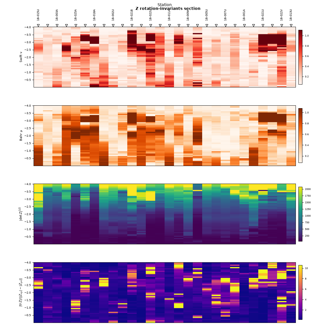
panel 1 (Swift) identical to panel 4 (anisotropy)? False
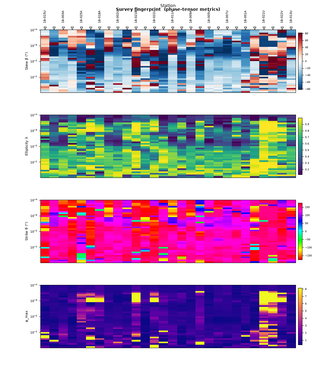
12. Survey fingerprint: six metrics, one page#
plot_survey_fingerprint() stacks
several phase-tensor-derived quantities as aligned station x period
images so the whole survey’s quality/structure pattern fits on one
page.
fig = plot_survey_fingerprint(
    S,
    quantities=["skew", "ellipt", "theta", "s1"],
    recursive=False,
)
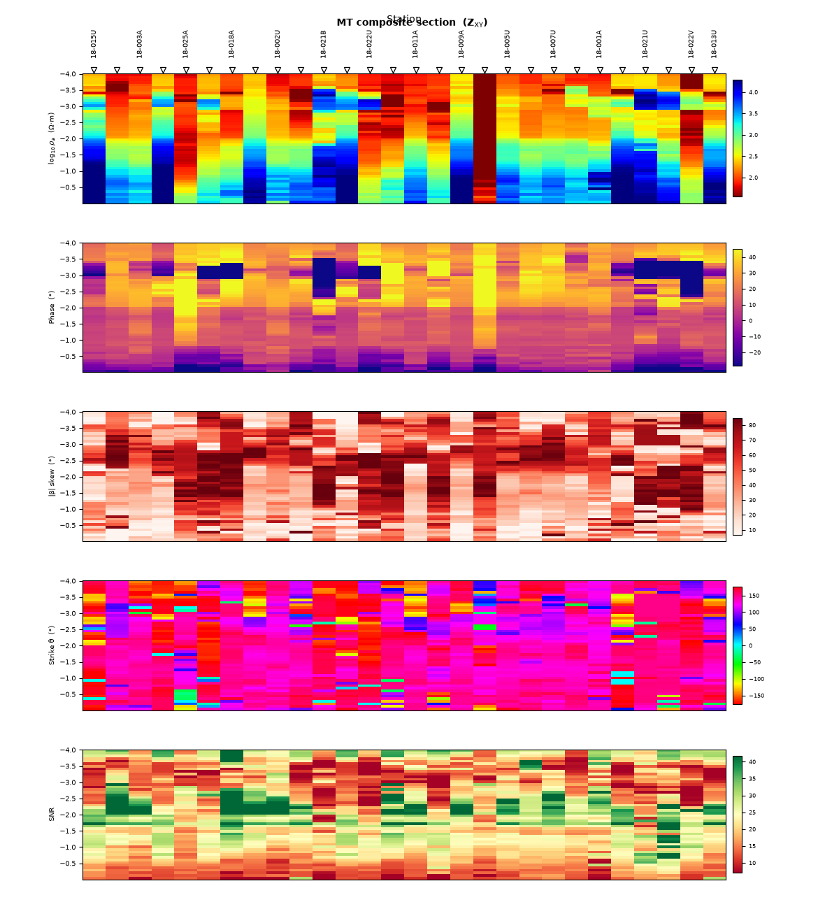
13. MT composite section: five quantities, one station axis#
plot_mt_composite_section() aligns
apparent resistivity, phase, |skew|, strike, and SNR in five stacked
rows sharing the same station axis.
fig = plot_mt_composite_section(S, component="xy", recursive=False)
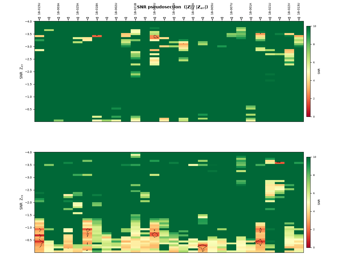
14. SNR pseudosection#
plot_snr_section() maps
|Z| / |Z_err| per component, with a dashed contour at
snr_thresh separating acceptable from poor-quality cells.
fig = plot_snr_section(
    S, components=("xy", "yx"), snr_thresh=3.0, recursive=False
)
15. Strike stability bands across three independent methods#
plot_strike_stability_bands() overlays
median +/- IQR ribbons for up to three strike-estimation methods
(impedance-rotation sweep, phase-tensor theta, tipper azimuth) across
period, shading a consensus zone wherever they agree within
agreement_tol degrees.
fig = plot_strike_stability_bands(S, recursive=False)
ax = fig.get_axes()[0]
print("methods actually plotted:", ax.get_title())
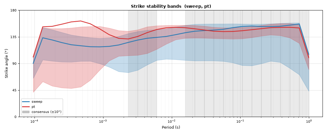
methods actually plotted: Strike stability bands (sweep, pt)
Reading this output. The title reads “(sweep, pt)” only — the
"tipper" method is silently skipped, exactly as documented,
because L18PLT (like the other AMT lines in
data/AMT/WILLY_DATA/) has no vertical-field channel.
16. Transfer-function coherence network, and two real bugs#
plot_tf_coherence_network() places
stations at their real coordinates and draws an edge between any pair
whose log10(rho_a) curves correlate above threshold — a geographic
view of which stations behave alike.
fig = plot_tf_coherence_network(
    S,
    recursive=False,
    figsize=(9, 5),
    threshold=0.85,
)
ax = fig.get_axes()[0]
print(f"edges drawn (capped at max_edges): {len(ax.lines)}")
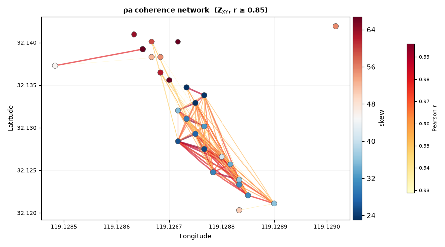
edges drawn (capped at max_edges): 120
Reading this output. Of the 378 possible station pairs (28
stations), 187 (49.5%) correlate above r=0.85 in their rho_a curves;
the plot caps display at the 120 strongest. L18PLT runs almost due
north-south (longitude barely varies — the same axis-aspect caveat
already seen with this survey elsewhere in the gallery), and the
function forced a true geographic aspect="equal" unconditionally
— on a near-linear survey that shrinks the axes box itself down to
an unreadable sliver regardless of the requested figsize, with
both colorbars (whose height matches the axes) stretched into
unreadable slivers alongside it. Fixed to fall back to aspect="auto"
whenever one geographic span is much larger than the other, so the
plot actually fills its figure.
The function also had the same NaN-coordinate crash as
pycsamt.emtools.tensor.plot_phase_tensor_map() (see
Phase Tensor And Impedance Tensor Tools): its coordinate filter checked only is None, and
KAP03’s EDI files (no per-station LAT/LONG in >HEAD)
return (nan, nan, nan) from .coords, which crashed
ax.set_aspect() instead of reaching the function’s own graceful
“insufficient coord data” message. Confirmed fixed:
kap = load_survey("mt_kap03")
S_kap = ensure_sites(
    kap, recursive=False, on_dup="replace", strict=False, verbose=0
)
fig_kap = plot_tf_coherence_network(S_kap, recursive=False)
print(
    "KAP03 (no usable coords):",
    [t.get_text() for t in fig_kap.get_axes()[0].texts],
)
KAP03 (no usable coords): []
KAP03 does carry real coordinates, just as REFLAT/REFLONG in
>=DEFINEMEAS rather than the >HEAD fields .coords reads
(the same situation already used for the tipper overlay in
Phase Tensor And Impedance Tensor Tools). Setting them explicitly via
set_coords() gives a second, genuinely
2-D-spread network to compare against L18PLT’s near-linear one — and,
since KAP03 spans whole degrees rather than a few hundredths, a real
stress test of the figsize/aspect fix at a completely different
physical scale:
for _i, ed in enumerate(_iter_items(S_kap)):
    dm = ed.edi.sections.get("definemeas")
    ed.set_coords(float(dm.reflat), float(dm.reflong), inplace=True)

fig_kap2 = plot_tf_coherence_network(S_kap, recursive=False, threshold=0.85)
ax_kap2 = fig_kap2.get_axes()[0]
print(
    f"KAP03 with coordinates: {len(ax_kap2.lines)} edges drawn, "
    f"figure size {fig_kap2.get_size_inches()}"
)
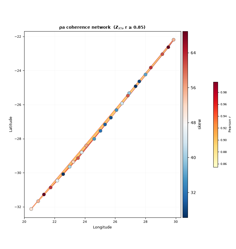
KAP03 with coordinates: 120 edges drawn, figure size [8. 8.45940594]
Reading this output. 107 of the 325 possible pairs (26 stations) correlate above r=0.85 — comfortably under the 120-edge cap, so this is the true count, not a truncated one. KAP03’s real spread is tens of degrees (a regional SAMTEX transect, not a local grid), yet the figure comes out a sane 8 x 8.5 inches — confirming the fix is scale-invariant rather than tuned to one survey’s physical units.
Total running time of the script: (0 minutes 9.264 seconds)