Bostick depth and CSUMT survey design (pycsamt.emtools.csumt)

pycsamt.emtools.csumt is built around one formula, the Bostick depth transform:

\[D(f) = 356 \sqrt{\rho_a(f) / f} \quad [\text{m}]\]

(Zhang et al. 2025, Measurement), and its inverse, used to pick the frequency that probes a target depth for a given background resistivity. The module has two distinct halves:

• Pure survey-planning functions — bostick_depth_from_rho(), frequency_for_depth(), frequency_schedule(), vertical_resolution_pair() — need no EDI data at all, only a resistivity estimate. They are for designing a CSUMT acquisition before going to the field.

• Sites-based analysis — bostick_depth(), vertical_resolution(), depth_coverage_table(), plot_depth_section() — apply the same transform to measured apparent resistivity from real EDI data. The Bostick transform itself does not care what frequency band it is given, so this example runs it on L18PLT/L22PLT (data/AMT/WILLY_DATA/, 1 Hz-10.4 kHz — the AMT band used throughout this documentation) even though CSUMT proper (Zhang et al. 2025) targets a much higher band, 9.6 kHz-614.4 kHz, for very shallow, high-resolution work. That contrast — CSUMT’s band only reaching a few tens of metres deep versus AMT’s much deeper reach — is itself one of the things this example demonstrates.

1. The Bostick relationship itself

No survey data needed yet: bostick_depth_from_rho() is a pure function of resistivity and frequency. Plotting it for a few resistivities across a wide frequency range shows the two things that control depth of investigation — lower frequency and higher resistivity both probe deeper.

import matplotlib.pyplot as plt
import numpy as np
from _datasets import load_survey

from pycsamt.emtools import (
    bostick_depth,
    bostick_depth_from_rho,
    depth_coverage_table,
    frequency_for_depth,
    frequency_schedule,
    plot_depth_section,
    vertical_resolution,
    vertical_resolution_pair,
)
from pycsamt.emtools.csumt import F_MAX_CSUMT, F_MIN_CSUMT

freq = np.logspace(-1, 6, 300)  # 0.1 Hz to 1 MHz - spans AMT and CSUMT
fig, ax = plt.subplots(figsize=(7, 5))
for rho, color in zip(
    [10.0, 100.0, 1000.0], ["#1f77b4", "#2ca02c", "#d62728"]
):
    ax.loglog(
        freq,
        bostick_depth_from_rho(rho, freq),
        color=color,
        label=rf"$\rho_a$ = {rho:g} $\Omega\cdot$m",
    )
ax.axvspan(
    F_MIN_CSUMT,
    F_MAX_CSUMT,
    color="0.85",
    zorder=0,
    label="CSUMT band (9.6 kHz-614.4 kHz)",
)
ax.set_xlabel("Frequency (Hz)")
ax.set_ylabel("Bostick depth D(f)  (m)")
ax.set_title(r"$D(f) = 356\sqrt{\rho_a/f}$")
ax.legend(fontsize=8)
ax.grid(True, which="both", alpha=0.3)

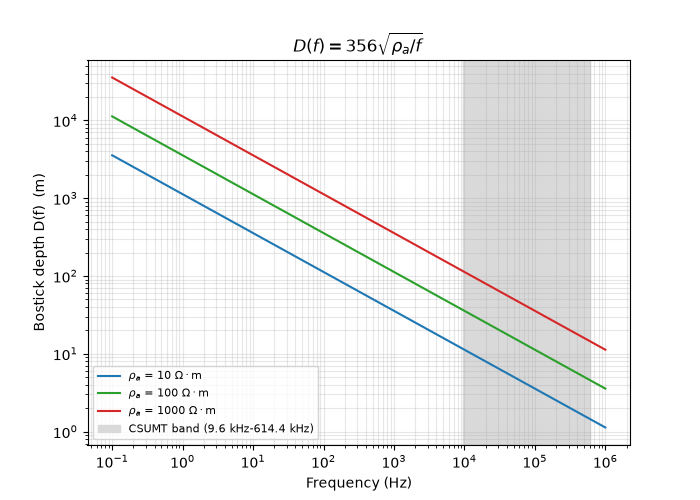
Reading this figure. Each line is straight in log-log space (slope -1/2, as the formula requires) and a decade of resistivity shifts the curve by exactly half a decade vertically. Inside the shaded CSUMT band, even at 1000 Ω·m the depth of investigation only spans about 14-115 m — this is fundamentally a shallow, near-surface method, not a substitute for lower-frequency AMT/MT when the target is deeper.

2. What depth range can a CSUMT survey actually reach?

For a fixed background resistivity, the CSUMT band’s own low/high frequency limits translate directly into a shallow and a deep bound on achievable depth.

rho_design = 300.0  # close to this survey's own median rho_a (below)
d_shallow = float(bostick_depth_from_rho(rho_design, F_MAX_CSUMT))
d_deep = float(bostick_depth_from_rho(rho_design, F_MIN_CSUMT))
print(
    f"At rho={rho_design:g} Ohm.m, CSUMT band resolves depths "
    f"{d_shallow:.1f}-{d_deep:.1f} m"
)

At rho=300 Ohm.m, CSUMT band resolves depths 7.9-62.9 m

3. Designing a frequency schedule for target depths

frequency_schedule() converts a list of target depths straight into transmitter frequencies, silently dropping any target that falls outside the instrument’s frequency band — a real trap if a target turns out to be deeper than the method can reach.

targets = np.array([10.0, 20.0, 35.0, 50.0, 65.0])
sched = frequency_schedule(targets, rho_design)
recovered_depth = bostick_depth_from_rho(rho_design, sched)

fig, ax = plt.subplots(figsize=(7, 4.5))
ax.scatter(
    targets,
    frequency_for_depth(targets, rho_design),
    s=60,
    facecolors="none",
    edgecolors="0.3",
    label="requested targets",
    zorder=3,
)
ax.scatter(
    recovered_depth,
    sched,
    s=40,
    color="#d62728",
    marker="x",
    label="kept in schedule",
    zorder=4,
)
ax.axhspan(F_MIN_CSUMT, F_MAX_CSUMT, color="0.9", zorder=0)
ax.set_yscale("log")
ax.set_xlabel("Depth (m)")
ax.set_ylabel("Frequency (Hz)")
targets_str = ", ".join(f"{t:g}" for t in targets)
ax.set_title(
    f"Frequency schedule for targets [{targets_str}] m  (rho={rho_design:g})"
)
ax.legend(fontsize=8)
ax.grid(True, alpha=0.3)

Reading this figure. Four of the five requested depths land inside the shaded band and come back out as scheduled frequencies. The 65 m target maps to about 9.0 kHz — just under the 9.6 kHz floor — so frequency_schedule() silently drops it; the function raises no warning, so always compare the length of its output against the number of targets you asked for.

Passing min_resolution_m inserts extra in-between frequencies wherever consecutive schedule entries would leave a resolution gap larger than that value:

sched_padded = frequency_schedule(targets, rho_design, min_resolution_m=5.0)
print(f"schedule without min_resolution_m: {len(sched)} frequencies")
print(f"schedule with min_resolution_m=5m: {len(sched_padded)} frequencies")

schedule without min_resolution_m: 4 frequencies
schedule with min_resolution_m=5m: 11 frequencies

4. Real data: one station’s Bostick depth vs. period

Switching to the sites-based half of the module: bostick_depth() reads the measured off-diagonal impedance and applies the same transform per frequency, for every station in a survey. _datasets.py is the shared loader introduced in the tf example.

survey = load_survey("amt_l18plt")
bd = bostick_depth(survey)
print(
    f"measured rho_a: {bd['rho_a_ohmm'].min():.1f}-{bd['rho_a_ohmm'].max():.1f} "
    f"Ohm.m (median {bd['rho_a_ohmm'].median():.0f})"
)

station = "18-001A"
d = bd[bd["station"] == station].sort_values("period_s")

fig, ax = plt.subplots(figsize=(7, 4.5))
ax.loglog(d["period_s"], d["depth_m"], "o-", ms=3)
ax.set_xlabel("Period (s)")
ax.set_ylabel("Bostick depth (m)")
ax.set_title(f"{station} — measured Bostick depth vs. period")
ax.grid(True, which="both", alpha=0.3)

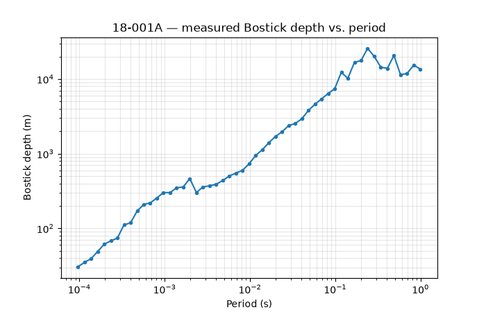
measured rho_a: 5.8-25388.5 Ohm.m (median 318)

Reading this figure. Depth grows roughly monotonically with period for this station, as expected, but not perfectly smoothly — each point uses that frequency’s own measured \(\rho_a\), not a smoothed background, so a noisy resistivity at one frequency can make its depth estimate dip below its shorter-period neighbour. That is a real, expected feature of the per-frequency transform, not a bug; the multi-station pseudo-section below shows the same behaviour is common across this whole line.

5. Per-station depth coverage

depth_coverage_table() collapses the whole band into one row per station: shallowest/deepest Bostick depth reached, and average resolution.

cov = depth_coverage_table(survey)
cov_sorted = cov.sort_values("depth_max_m")

fig, ax = plt.subplots(figsize=(7, 6))
ax.barh(
    cov_sorted["station"], cov_sorted["depth_max_m"] / 1000.0, color="#1f77b4"
)
ax.set_xlabel("Deepest Bostick depth reached (km)")
ax.tick_params(axis="y", labelsize=6)
ax.set_title("L18PLT — per-station depth coverage")
fig.tight_layout()

print(
    f"shallowest max-depth station: {cov_sorted.iloc[0]['station']} "
    f"({cov_sorted.iloc[0]['depth_max_m']:.0f} m)"
)
print(
    f"deepest max-depth station: {cov_sorted.iloc[-1]['station']} "
    f"({cov_sorted.iloc[-1]['depth_max_m']:.0f} m)"
)

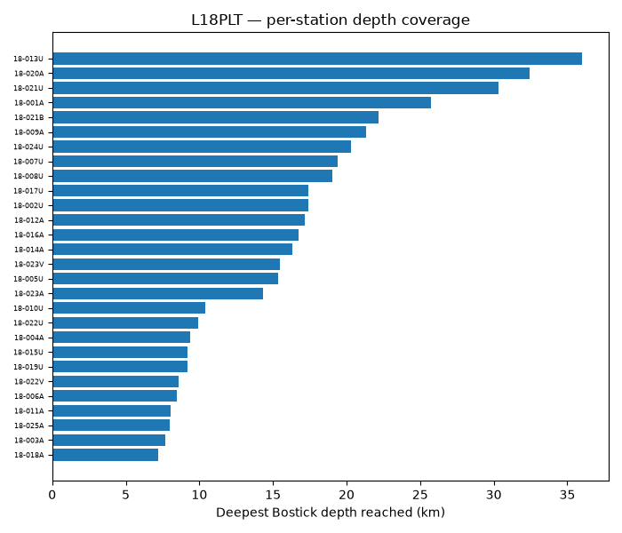
shallowest max-depth station: 18-018A (7228 m)
deepest max-depth station: 18-013U (36009 m)

Reading this figure. All 28 stations share the same 53-frequency schedule (1-10,400 Hz), yet their achieved Bostick depth still spans roughly a 5x range station to station (about 7.2 km up to 36 km at the extremes) — purely because Bostick depth also depends on each station’s own measured resistivity, not just the frequency. A uniform acquisition schedule does not guarantee uniform depth of investigation across a line.

6. Bostick depth pseudo-section

plot_depth_section() is the module’s headline view: every station’s full depth-vs-period profile from step 4, side by side.

plot_depth_section(survey)

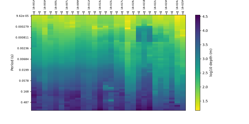
<Axes: title={'center': 'Bostick Depth Section  D = 356√(ρ_a / f)'}, xlabel='Station', ylabel='Period (s)'>

Reading this figure. Depth (colour) generally warms toward the bottom of the section (longer period) for most stations, consistent with step 4, but the banding is uneven column to column — some stations reach much deeper colours near the bottom than their neighbours, matching the wide spread in maximum depth already seen in the per-station ranking above.

7. Advanced: does resolution really coarsen with depth?

vertical_resolution() gives the depth gap between every pair of adjacent frequencies. Binning it by depth across all 28 stations tests whether resolution coarsens with depth the way the Bostick formula implies, and overlaying the purely analytical vertical_resolution_pair() curve (built from nothing but this line’s own median resistivity swept across its frequency range) checks whether the idealised formula matches what the real, noisy data show.

vr = vertical_resolution(survey)
vr["mid_depth"] = 0.5 * (vr["depth_lo_m"] + vr["depth_hi_m"]).abs()
bins = np.logspace(0.5, 4, 12)
centers = np.sqrt(bins[:-1] * bins[1:])
bin_idx = np.digitize(vr["mid_depth"].abs(), bins)
binned = (
    vr.groupby(bin_idx)["delta_depth_m"]
    .apply(lambda s: np.median(np.abs(s)))
    .loc[lambda s: (s.index >= 1) & (s.index <= len(centers))]
)

rho_med = float(bd["rho_a_ohmm"].median())
f_sweep = np.logspace(
    np.log10(bd["freq_hz"].min()), np.log10(bd["freq_hz"].max()), 40
)
analytic_depth, analytic_res = [], []
for f_lo, f_hi in zip(f_sweep[:-1], f_sweep[1:]):
    analytic_depth.append(
        float(
            np.sqrt(
                bostick_depth_from_rho(rho_med, f_lo)
                * bostick_depth_from_rho(rho_med, f_hi)
            )
        )
    )
    analytic_res.append(vertical_resolution_pair(rho_med, f_lo, f_hi))

fig, ax = plt.subplots(figsize=(7, 5))
ax.loglog(
    centers[binned.index - 1],
    binned.values,
    "o-",
    label="measured (median, binned)",
)
ax.loglog(
    analytic_depth,
    analytic_res,
    "--",
    color="0.3",
    label=rf"analytic, $\rho$={rho_med:.0f} $\Omega\cdot$m",
)
ax.set_xlabel("Depth (m)")
ax.set_ylabel(r"Vertical resolution $\Delta D$ (m)")
ax.set_title("L18PLT — resolution coarsens with depth")
ax.legend(fontsize=8)
ax.grid(True, which="both", alpha=0.3)

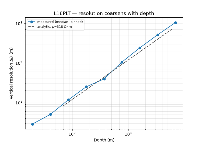
Reading this figure. The measured, binned resolution grows by roughly two and a half orders of magnitude from the shallowest to the deepest bin (about 3 m near the surface to over 2 km at depth) — a real, monotonic trend, not noise. It tracks the analytic curve built from nothing but the median resistivity reasonably well, which is itself a useful check: if a real line’s measured resolution trend diverged sharply from the analytic curve for its own median resistivity, that would flag a resistivity distribution too heterogeneous for a single background value to describe well.

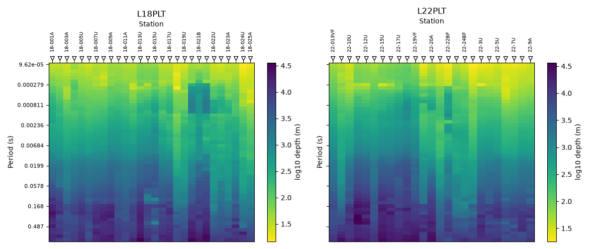
8. Advanced: comparing two lines of the same survey

As in the anisotropy example, ax lets two lines share one figure.

survey22 = load_survey("amt_l22plt")

fig, (axa, axb) = plt.subplots(1, 2, figsize=(12, 5), sharey=True)
plot_depth_section(survey, ax=axa)
axa.set_title("L18PLT")
plot_depth_section(survey22, ax=axb)
axb.set_title("L22PLT")
fig.tight_layout()

cov22 = depth_coverage_table(survey22)
print(f"L18PLT mean deepest-depth: {cov['depth_max_m'].mean():.0f} m")
print(f"L22PLT mean deepest-depth: {cov22['depth_max_m'].mean():.0f} m")

L18PLT mean deepest-depth: 16171 m
L22PLT mean deepest-depth: 18017 m

Reading this figure. The two neighbouring lines look qualitatively similar and their mean achieved depths are within about 10% of each other (L18PLT ≈ 16.2 km vs L22PLT ≈ 18.0 km, both driven by a handful of very high-resistivity, low-frequency outlier estimates rather than a literal, trustworthy 16-18 km depth of investigation) — reasonable agreement for two lines from the same survey, and a reminder that Bostick depth is a fast qualitative 1-D transform, not a substitute for real 2-D/3-D inversion when the absolute depth number matters.