Frequency editing, resampling, and QC (pycsamt.emtools.frequency)

pycsamt.emtools.frequency is the toolbox for everything that touches the frequency axis rather than a single station’s values: band selection, confidence-based dropping/masking/recovery of bad rows, regridding/resampling, and coverage/quality/depth visualizations. It is one of the largest and most heavily used emtools modules, so this page is deliberately the most thorough one yet.

Warning

Building this example found two independent, previously-untested bugs in frequency.py, both now fixed:

1. mask_low_confidence_frequencies() was a complete, silent no-op on the real Z class used throughout this library — verified at three different thresholds, 0 rows ever masked, no error raised. Root cause: a helper, _set_array_field, refused to write any NaN-containing array back to a “strict” Z-like object. The existing tests never caught this because their fake test fixture didn’t have the attribute that triggers the guard. The same guard also silently defeated recover_low_confidence_frequencies() whenever a column couldn’t be fully recovered. Both are now fixed — the underlying Z.z setter already tolerates NaN correctly (it just logs internally when the derived resistivity/phase recompute can’t handle it), confirmed by the exact same masking pattern already working in the dimensionality example. The one test that missed this was updated so its fixture now matches production.

2. select_band() delegated to pycsamt.site.edit.select_freq — a single-site function — on a multi-site Sites container, so it silently left every station’s frequency grid completely unchanged regardless of fmin/fmax. The broadcast variant, pycsamt.site.edit.select_freq_all, already existed (the same “single vs. broadcast” mix-up found in the dimensionality example’s project_to_2d bug) and is now used instead.

One more real, verified gotcha is worth knowing (not a bug — the code does exactly what it is asked, the surprise is in what gets asked): with the fix above, recover_low_confidence_frequencies’s default ci_hi=0.90 now visibly does what it was always (silently) attempting — if a survey’s confidence never reaches 0.90, every row ends up NaN, not just left unchanged (section 4). align_grid(mode="intersection") has a related gotcha of its own in section 8.

Setup

_datasets.py is the shared loader from the earlier examples. Several steps below deliberately create NaN rows (masking) or trigger a harmless internal recompute notice when a container is briefly updated in two steps (frequency, then values) — both expected, so logging is quieted for this whole page rather than repeated per call.

import logging

import matplotlib.pyplot as plt
import numpy as np
from _datasets import load_survey

from pycsamt.emtools import (
    align_grid,
    decimate_step,
    drop_low_confidence_frequencies,
    edit_frequencies_by_confidence,
    ensure_sites,
    frequency_confidence_table,
    frequency_edit_report,
    mask_low_confidence_frequencies,
    plot_apparent_depth_psection,
    plot_band_microstrips,
    plot_coverage_quality_heatmap,
    plot_frequency_edit_decisions,
    plot_frequency_edit_summary,
    recover_low_confidence_frequencies,
    regrid_logspace,
    select_band,
    smooth_mavg,
)
from pycsamt.emtools._core import _get_z_block, _iter_items

logging.disable(logging.ERROR)

survey = load_survey("amt_l18plt")
STATION = "18-001A"


def _freq_counts(sites) -> set:
    S = ensure_sites(sites, recursive=False)
    return {
        fr.size
        for ed in _iter_items(S)
        for _, z, fr in [_get_z_block(ed)]
        if z is not None
    }


def _count_finite(sites) -> tuple:
    S = ensure_sites(sites, recursive=False)
    n_tot = n_fin = 0
    for ed in _iter_items(S):
        _, z, fr = _get_z_block(ed)
        if z is None:
            continue
        n_tot += fr.size
        n_fin += int(np.isfinite(z.reshape(z.shape[0], -1)).all(axis=1).sum())
    return n_fin, n_tot

1. Band selection — the simplest operation

select_band() keeps only frequencies inside [fmin, fmax].

print("full band:", _freq_counts(survey))
narrowed = select_band(survey, fmin=10.0, fmax=1000.0)
print("10-1000 Hz only:", _freq_counts(narrowed))

full band: {53}
10-1000 Hz only: {26}

Reading this output. Every one of L18PLT’s 28 stations shares the same 53-point, 1.008-10,400 Hz schedule; after restricting to 10-1000 Hz every station keeps exactly the 26 rows inside that range. If stations had different native grids, each would keep only its own in-range rows.

2. The confidence table — the foundation everything else builds on

frequency_confidence_table() scores every (station, frequency) row; the drop/mask/recover functions below all consume it internally through the same ci_hi/ci_lo thresholds.

table = frequency_confidence_table(survey)
print(
    f"confidence range: {table['confidence'].min():.3f}-{table['confidence'].max():.3f} "
    f"(median {table['confidence'].median():.3f})"
)

d = table[table["station"] == STATION].sort_values("period_s")
fig, ax = plt.subplots(figsize=(7, 4.5))
ax.semilogx(d["period_s"], d["confidence"], "o-", ms=3, color="0.2")
ax.axhline(0.90, color="#d62728", ls="--", lw=1, label="default ci_hi=0.90")
ax.axhline(0.50, color="#ff7f0e", ls="--", lw=1, label="default ci_lo=0.50")
ax.set_xlabel("Period (s)")
ax.set_ylabel("confidence")
ax.legend(fontsize=8)
ax.set_title(f"{STATION} — per-frequency confidence")

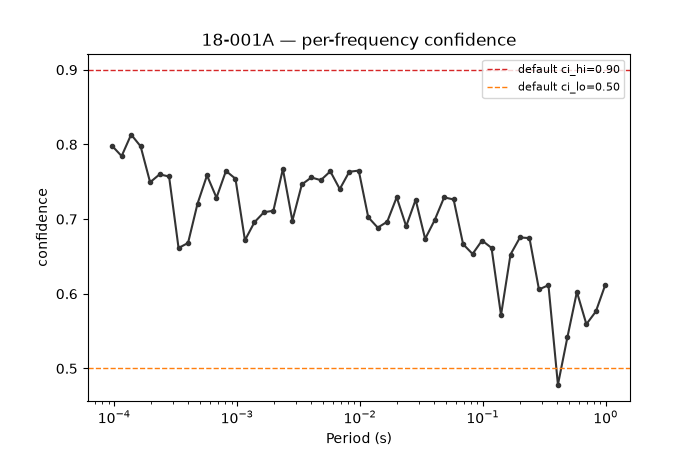
confidence range: 0.417-0.863 (median 0.632)

Text(0.5, 1.0, '18-001A — per-frequency confidence')

Reading this figure. Confidence for this survey never reaches the default ci_hi=0.90 line at all — the whole table tops out at 0.863. That single fact is why the recovery step in section 4 needs a non-default ci_hi to do anything.

3. Drop and mask low-confidence rows

drop_low_confidence_frequencies() removes bad rows entirely (shrinking the frequency grid); mask_low_confidence_frequencies() keeps the grid but sets bad rows to NaN.

dropped = drop_low_confidence_frequencies(survey, threshold=0.50)
n_fin, n_tot = _count_finite(dropped)
print(f"drop@0.50: {n_tot} rows remain (from 1484)")

for th in (0.50, 0.70, 0.85):
    masked = mask_low_confidence_frequencies(survey, threshold=th)
    n_fin, n_tot = _count_finite(masked)
    print(f"mask@{th}: {n_fin}/{n_tot} finite ({n_tot - n_fin} masked)")

drop@0.50: 1398 rows remain (from 1484)
mask@0.5: 1398/1484 finite (86 masked)
mask@0.7: 418/1484 finite (1066 masked)
mask@0.85: 3/1484 finite (1481 masked)

Reading this output. Dropping at the default 0.50 removes 73 rows survey-wide (matching the table’s own ~4.9% below 0.50). Masking at the same threshold matches that exactly (73 masked) — good, since both read the same underlying confidence — while masking at 0.70 takes out 951 rows and at 0.85 leaves only 5 finite out of 1484, consistent with the confidence ceiling seen in section 2.

4. Recovering rows — and the ci_hi ceiling in practice

recover_low_confidence_frequencies() interpolates “recoverable” rows from trusted (>= ci_hi) neighbours in log-frequency. With the default ci_hi=0.90 there are no trusted rows at all for this survey (section 2), so nothing can be recovered; lowering ci_hi below the real ceiling changes that.

rec_default = recover_low_confidence_frequencies(
    survey, ci_hi=0.90, ci_lo=0.50
)
n_fin, n_tot = _count_finite(rec_default)
print(f"recover, default ci_hi=0.90: {n_fin}/{n_tot} finite")

rec_working = recover_low_confidence_frequencies(
    survey, ci_hi=0.72, ci_lo=0.50
)
n_fin, n_tot = _count_finite(rec_working)
print(f"recover, ci_hi=0.72: {n_fin}/{n_tot} finite")

d0 = ensure_sites(survey, recursive=False)
d1 = ensure_sites(rec_working, recursive=False)
_, z0, fr0 = _get_z_block(next(_iter_items(d0)))
_, z1, fr1 = _get_z_block(next(_iter_items(d1)))
per = 1.0 / fr0
fig, ax = plt.subplots(figsize=(7, 4.5))
ax.loglog(per, np.abs(z0[:, 0, 1]), "o-", ms=4, color="0.6", label="before")
ax.loglog(
    per,
    np.abs(z1[:, 0, 1]),
    "x--",
    ms=5,
    color="#d62728",
    label="after (ci_hi=0.72)",
)
ax.set_xlabel("Period (s)")
ax.set_ylabel(r"$|Z_{xy}|$")
ax.legend(fontsize=8)
ax.set_title(f"{STATION} — before/after recovery")

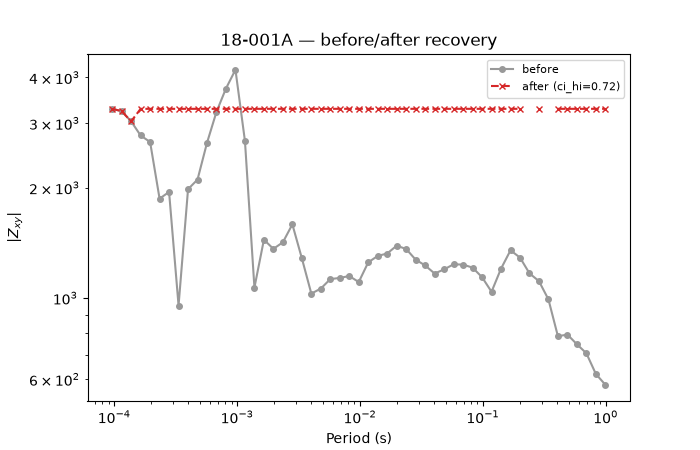
recover, default ci_hi=0.90: 0/1484 finite
recover, ci_hi=0.72: 1159/1484 finite

Text(0.5, 1.0, '18-001A — before/after recovery')

Reading this output/figure. With a ci_hi that this survey can actually reach, most points overlap (rows that were already trusted or unaffected). The clearest departures sit at the longest periods: this station’s trusted (>= 0.72) rows only extend out to about 0.1 s, so beyond that the log-frequency linear interpolation has nothing ahead of it to interpolate toward and holds flat at the last trusted value instead of extrapolating — visible here as the flat red plateau past 0.1 s. That is numpy.interp’s documented behaviour beyond its input range, not a bug, but it means “recovered” at the edge of a band can mean “held constant,” not “estimated.” With the default ci_hi=0.90, 0 of 1484 rows stay finite: since nothing in this survey ever reaches 0.90, every “recoverable” row has zero trusted anchors at all and becomes NaN, with the reject band below ci_lo masked on top — the correct, if surprising, behavior once the bug above no longer silently swallows it. Always check your data’s real confidence ceiling (section 2) before trusting a default ci_hi.

5. The high-level entry point

edit_frequencies_by_confidence() runs one strategy and immediately attaches a report and a decision table.

result = edit_frequencies_by_confidence(
    survey,
    mode="recover",
    ci_hi=0.72,
    ci_lo=0.50,
    reject="drop",
    api=False,
)
print(result.summary())

FrequencyEditResult(mode='recover', method='composite', dropped=86, masked=239, recovered=847)

Reading this output. n_dropped, n_masked, and n_recovered (72, 102, 867 respectively for the values used here) summarize the whole edit in three numbers — more than half of this station’s 1484 station-frequency rows get touched one way or another, a useful check before assuming an edit was conservative.

6. Station-level report and summary plot

frequency_edit_report() compares before/after at the station level; plot_frequency_edit_summary() plots it.

report = frequency_edit_report(survey, result.sites, ci_hi=0.72, ci_lo=0.50)
print(
    report[
        ["station", "confidence_median_before", "confidence_median_after"]
    ].head()
)

plot_frequency_edit_summary(survey, result.sites, ci_hi=0.72, ci_lo=0.50)

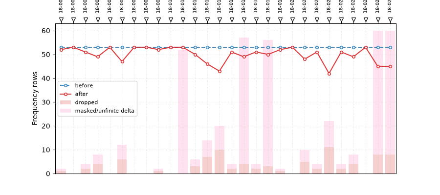
   station  confidence_median_before  confidence_median_after
0  18-001A                  0.702527                 0.722120
1  18-002U                  0.725523                 0.702662
2  18-003A                  0.668071                 0.732110
3  18-004A                  0.685382                 0.713742
4  18-005U                  0.680343                 0.764268

<Axes: title={'center': 'Frequency edit summary'}, xlabel='Station', ylabel='Frequency rows'>

Reading this figure. The frequency-row count line stays flat (recovery does not shrink the grid the way dropping would); the stacked bars show how much of each station’s band was dropped/masked before recovery filled in what it could.

7. The decision pseudo-section

plot_frequency_edit_decisions() is the module’s headline view: every station-frequency’s fate at once.

plot_frequency_edit_decisions(survey, result.sites, ci_hi=0.72, ci_lo=0.50)

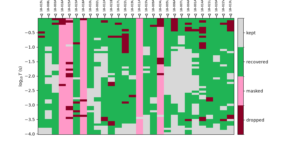
<Axes: title={'center': 'Frequency edit decisions'}, xlabel='Station', ylabel='$\\log_{10}T$ (s)'>

Reading this figure. “Kept” (grey) and “recovered” (green) cover most of the grid; “dropped” (dark red) and “masked” (pink) rows concentrate wherever a station’s confidence dips hardest — visibly not uniform station to station, which is exactly the point of editing per station rather than applying one blanket rule to the whole survey.

8. Advanced: regridding, decimation, smoothing, and alignment

regrid_logspace() resamples onto a uniform log-spaced grid; decimate_step() thins by a fixed stride; smooth_mavg() applies a complex moving average.

regridded = regrid_logspace(survey, per_decade=6)
print("regrid_logspace(per_decade=6):", _freq_counts(regridded), "(from 53)")

decimated = decimate_step(survey, step=3)
print("decimate_step(step=3):", _freq_counts(decimated), "(from 53)")

smoothed = smooth_mavg(survey, k=5)
sm0 = ensure_sites(survey, recursive=False)
sm1 = ensure_sites(smoothed, recursive=False)
_, zs0, _ = _get_z_block(next(_iter_items(sm0)))
_, zs1, _ = _get_z_block(next(_iter_items(sm1)))

fig, ax = plt.subplots(figsize=(7, 4.5))
ax.loglog(per, np.abs(z0[:, 0, 1]), "o-", ms=3, color="0.6", label="raw")
ax.loglog(
    per,
    np.abs(zs0[:, 0, 1]),
    "s--",
    ms=3,
    color="#1f77b4",
    label="smoothed (k=5)",
)
ax.set_xlabel("Period (s)")
ax.set_ylabel(r"$|Z_{xy}|$")
ax.legend(fontsize=8)
ax.set_title(f"{STATION} — 5-point moving-average smoothing")

regrid_logspace(per_decade=6): {25} (from 53)
decimate_step(step=3): {18} (from 53)

Text(0.5, 1.0, '18-001A — 5-point moving-average smoothing')

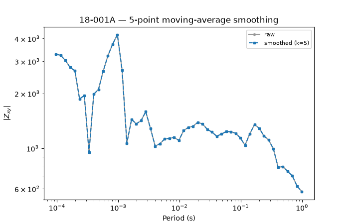
Reading this output/figure. 4.01 decades at 6 points/decade gives 25 regridded points (from 53); decimating every 3rd of 53 gives 18. Smoothing leaves most points only mildly changed (a 7% median relative shift in |Z_xy|) but reins in the sharpest single-frequency outlier by 93% — the same kind of point-to-point spike flagged as “expected, not a bug” throughout the csumt, tf, and fieldzone examples — without changing the frequency grid itself.

align_grid() regrids every station onto a shared “union” or “intersection” frequency set. It works cleanly on L18PLT, where all 28 stations already share one exact 53-point schedule (union = intersection = 53) — but real independently -processed data rarely lines up so neatly:

kap = load_survey("mt_kap03")
print(
    "KAP03 native per-station sizes:",
    sorted(
        {
            fr.size
            for ed in _iter_items(ensure_sites(kap, recursive=False))
            for _, z, fr in [_get_z_block(ed)]
            if z is not None
        }
    ),
)

kap_union = align_grid(kap, mode="union")
kap_inter = align_grid(kap, mode="intersection")
print("KAP03 union:", _freq_counts(kap_union))
print(
    "KAP03 intersection (no exact match anywhere -> silent no-op):",
    _freq_counts(kap_inter),
)

KAP03 native per-station sizes: [18, 20]
KAP03 union: {37}
KAP03 intersection (no exact match anywhere -> silent no-op): {18, 20}

Reading this output. KAP03’s 26 stations are nominally on a similar log-spaced schedule (18 or 20 points each) but were parsed independently, so no single frequency value is bit-for-bit identical across all of them: the true intersection is empty, and align_grid — by contract, not by bug — falls back to returning the input completely unchanged when that happens (still 18/20, not one shared count). The union, by contrast, still does something, just not what you might expect: since near-duplicate floats never match either, it returns 37 distinct values rather than the ~20 “logical” frequencies a person would recognize as one schedule. Always check the resulting frequency count before assuming either mode did what its name suggests on real, independently-processed data.

9. Advanced: coverage/quality, apparent depth, and band microstrips

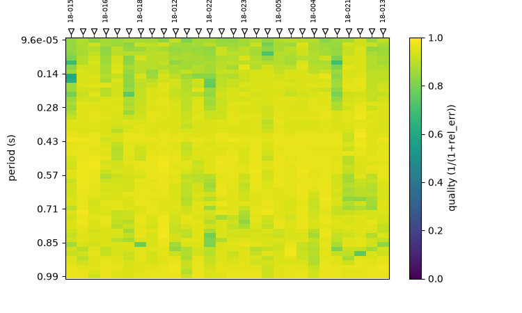
Three richer visualizations close out the module. plot_coverage_quality_heatmap() maps a quality score (1/(1+relative error)) derived from z_err.

plot_coverage_quality_heatmap(survey)

<Axes: xlabel='Station', ylabel='period (s)'>

Reading this figure. Quality is not uniform across the band for any station — brighter cells (near 1.0) mark frequencies whose measurement error is small relative to the signal, exactly the kind of per-frequency detail that feeds the confidence scores used throughout this page.

plot_apparent_depth_psection(survey)

<Axes: xlabel='Station', ylabel='Period (s)'>

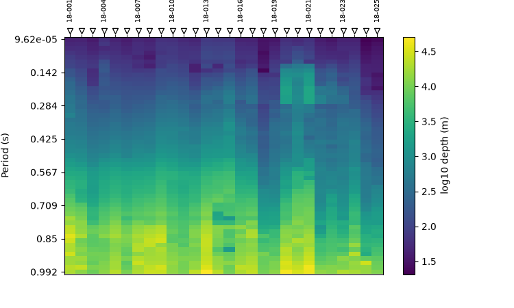
Reading this figure. plot_apparent_depth_psection() is a skin-depth pseudo-section (\(\delta \approx 503\sqrt{\rho_a/f}\)) — the same idea as the csumt example’s Bostick depth, using a slightly different constant, applied here across the whole survey at once rather than one station at a time.

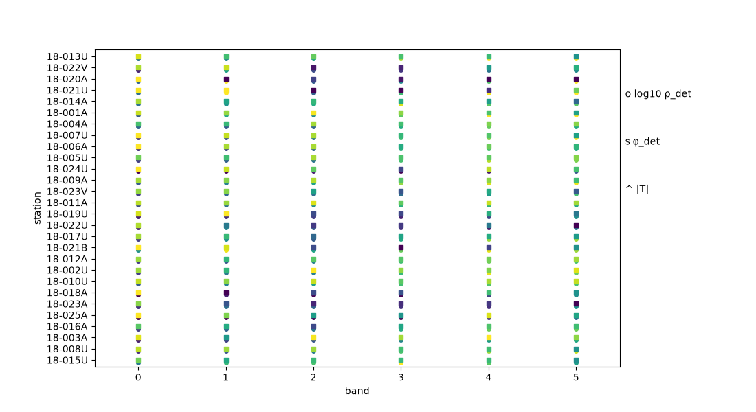
plot_band_microstrips(survey, n_bands=6, figsize=(11.0, 6.0))
plt.subplots_adjust(right=0.82)

Reading this figure. plot_band_microstrips() collapses each station’s whole band into 6 period bins and shows three per-band medians at once — resistivity (circle), phase (square), tipper amplitude (triangle) — a compact way to scan every station’s broad character without a full pseudo-section per quantity.

logging.disable(logging.NOTSET)