Phased-array CSAMT transmitter design (pycsamt.emtools.source_array)

pycsamt.emtools.source_array is the one emtools module with no site or EDI data at all: it implements the phased-array transmitting source (PAS) antenna theory of Fan, Zhang & Wang (2022) — element pattern, array factor, beam steering, directivity, and SNR gain for an N-element linear array of CSAMT dipole sources, replacing the traditional single-dipole antenna source (SDAS). Every number below comes from the formulas themselves at representative CSAMT frequencies and resistivities, not from a bundled survey.

1. The single-dipole (SDAS) element pattern

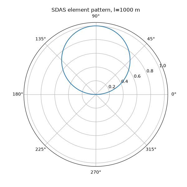
wavenumber() returns the effective earth wavenumber for CSAMT — not the free-space one, which is meaningless at these frequencies — and sdas_element_pattern() is the far-field pattern of one finite-length dipole (eq. 7): a null along the dipole axis, maximum broadside.

import matplotlib.pyplot as plt
import numpy as np

from pycsamt.emtools import (
    array_factor,
    beam_steer,
    pas_pattern,
    plot_radiation_pattern,
    sdas_directivity,
    sdas_element_pattern,
    snr_gain_db,
    steering_angles,
    wavenumber,
)

freq, rho = 8.0, 300.0
k_earth = wavenumber(freq, rho)
k_free = wavenumber(freq)
print(
    f"earth wavelength at {freq:g} Hz, {rho:g} ohm.m: {2 * np.pi / k_earth:,.0f} m"
)
print(f"free-space wavelength at {freq:g} Hz: {2 * np.pi / k_free:,.0f} m")

theta = np.linspace(0.0, 180.0, 721)
F = sdas_element_pattern(theta, l=1000.0, k=k_earth)
print(f"F(0 deg)={F[0]:.2e}  F(90 deg)={F[360]:.3f}  F(180 deg)={F[-1]:.2e}")

fig, ax = plt.subplots(subplot_kw={"projection": "polar"}, figsize=(6, 6))
ax.plot(np.deg2rad(theta), F)
ax.set_title("SDAS element pattern, l=1000 m")

earth wavelength at 8 Hz, 300 ohm.m: 19,365 m
free-space wavelength at 8 Hz: 37,474,057 m
F(0 deg)=0.00e+00  F(90 deg)=1.000  F(180 deg)=0.00e+00

Text(0.5, 1.0571188071188073, 'SDAS element pattern, l=1000 m')

Reading this output/figure. At 8 Hz over a 300 Ω·m half-space, the earth wavelength is about 19.4 km — the free-space wavelength at the same frequency would be roughly 37,470 km, useless for antenna design at CSAMT scale, which is exactly why the module insists on the earth wavenumber for anything array-related. The 1000 m dipole’s pattern is essentially zero along its own axis (0°/180°) and exactly 1.0 broadside (90°) — the classic figure-eight dipole shape, confirmed numerically rather than just visually.

2. Array factor: gentle at low frequency, no true nulls yet

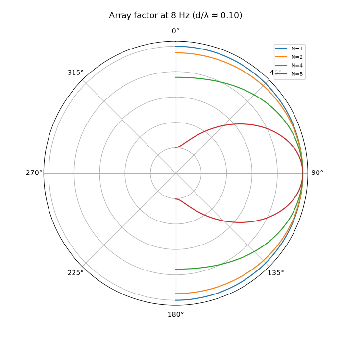
array_factor() (eq. 19) describes how N co-linear elements interfere. At 8 Hz with a realistic 2 km element spacing, the spacing is only about a tenth of the earth wavelength — far too small, at this frequency, for the array to form the sharp nulls a textbook antenna array would show at radio frequencies.

d = 2000.0
theta_b = np.linspace(-90.0, 90.0, 721)
print(f"d / wavelength at {freq:g} Hz: {d / (2 * np.pi / k_earth):.3f}")

patterns_lf = [array_factor(theta_b, N, d, k_earth) for N in (1, 2, 4, 8)]
plot_radiation_pattern(
    theta_b,
    patterns_lf,
    labels=[f"N={n}" for n in (1, 2, 4, 8)],
    title=f"Array factor at {freq:g} Hz (d/λ ≈ 0.10)",
)

d / wavelength at 8 Hz: 0.103

<PolarAxes: title={'center': 'Array factor at 8 Hz (d/λ ≈ 0.10)'}>

Reading this figure. N=1 is a perfect, undirected semicircle at radius 1 — one element has no array to interfere with. Adding elements narrows the main lobe somewhat, but none of these curves develop a true zero: at this frequency the array is simply too small, in wavelengths, for classical nulls to form within \(\pm 90^\circ\), even at N=8.

3. The same array at a higher CSAMT frequency

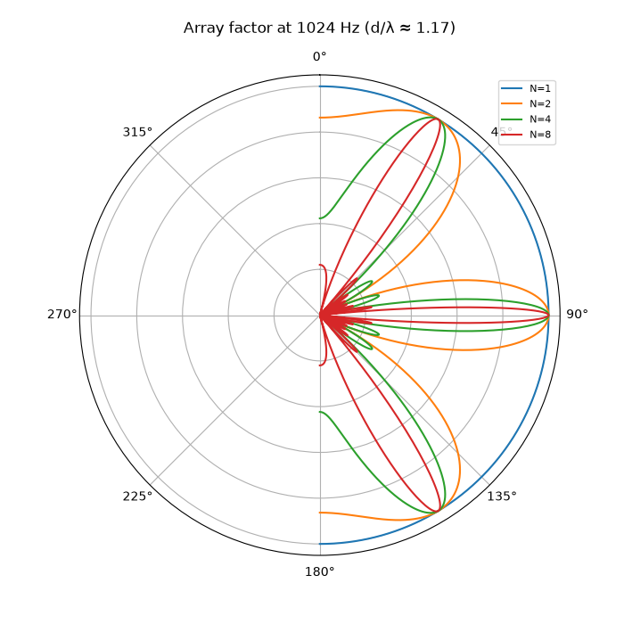
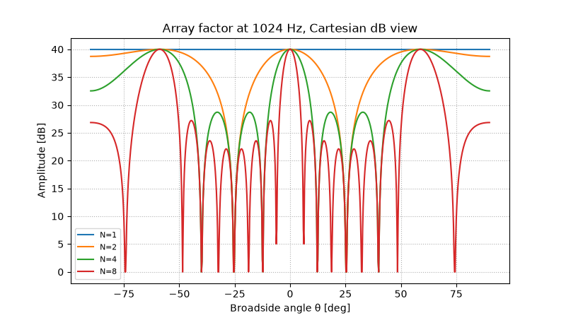
Raising the frequency to 1024 Hz (still an ordinary CSAMT frequency) shrinks the earth wavelength to about 1.7 km — now shorter than the 2 km element spacing — and the same physical array behaves very differently.

freq_hf = 1024.0
k_hf = wavenumber(freq_hf, rho)
wl_hf = 2 * np.pi / k_hf
print(
    f"earth wavelength at {freq_hf:g} Hz: {wl_hf:.0f} m;  d/wavelength = {d / wl_hf:.3f}"
)

patterns_hf = [array_factor(theta_b, N, d, k_hf) for N in (1, 2, 4, 8)]
plot_radiation_pattern(
    theta_b,
    patterns_hf,
    labels=[f"N={n}" for n in (1, 2, 4, 8)],
    title=f"Array factor at {freq_hf:g} Hz (d/λ ≈ 1.17)",
)

fig, ax = plt.subplots(figsize=(8, 4.5))
plot_radiation_pattern(
    theta_b,
    patterns_hf,
    labels=[f"N={n}" for n in (1, 2, 4, 8)],
    polar=False,
    log_scale=True,
    ax=ax,
    title=f"Array factor at {freq_hf:g} Hz, Cartesian dB view",
)

• 
• 

earth wavelength at 1024 Hz: 1712 m;  d/wavelength = 1.168

<Axes: title={'center': 'Array factor at 1024 Hz, Cartesian dB view'}, xlabel='Broadside angle θ [deg]', ylabel='Amplitude [dB]'>

Reading this figure. With the element spacing now larger than one wavelength, real nulls and side lobes appear even for N=2, and N=8 shows a narrow main lobe flanked by several clear side lobes — the textbook array-factor shape that section 2’s lower frequency never produced. A phased array’s directionality on a real CSAMT line is therefore not a fixed property of the hardware layout alone: it depends on which frequency in the sweep is being transmitted.

4. Beam steering — and a grating lobe warning

beam_steer() computes the inter-element phase shift needed to point the main lobe at a target angle (eq. 23); steering_angles() solves for every angle satisfying the array’s periodicity — including unwanted grating lobes.

beta_20 = beam_steer(20.0, d, k_hf)
af_steered = array_factor(theta_b, 4, d, k_hf, beta=beta_20)
peak_angle = theta_b[np.argmax(af_steered)]
print(
    f"target 20 deg -> beta={beta_20:.4f} rad, actual peak at {peak_angle:.2f} deg"
)

angles = steering_angles(4, d, k_hf, beta_20, n_range=3)
print("all main-lobe angles (target + grating lobes):", angles)

target 20 deg -> beta=-2.5110 rad, actual peak at 20.00 deg
all main-lobe angles (target + grating lobes): [-30.917035  20.      ]

Reading this output. The steered peak lands at 20.0°, matching the target essentially exactly. But steering_angles() reports a second angle at -30.9° — a genuine grating lobe, a direct consequence of section 3’s \(d/\lambda\approx 1.17\) spacing. At 8 Hz (section 2), the same steering command produces no grating lobe at all within \(\pm 90^\circ\), because the array is too small in wavelengths for one to exist. Element spacing chosen for one frequency can silently misbehave at another.

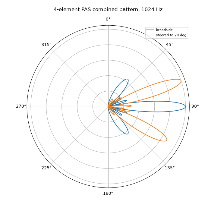
5. The combined PAS pattern

pas_pattern() multiplies the element pattern (section 1) by the array factor (sections 2-4) to get the total far-field pattern a real N-element PAS would radiate.

pat_broadside = pas_pattern(theta_b, N=4, d=d, k=k_hf, beta=0.0, l=1000.0)
pat_steered = pas_pattern(theta_b, N=4, d=d, k=k_hf, beta=beta_20, l=1000.0)
plot_radiation_pattern(
    theta_b,
    [pat_broadside, pat_steered],
    labels=["broadside", "steered to 20 deg"],
    title=f"4-element PAS combined pattern, {freq_hf:g} Hz",
)

<PolarAxes: title={'center': '4-element PAS combined pattern, 1024 Hz'}>

Reading this figure. The combined pattern keeps the array factor’s narrow main lobe from section 3-4 while the element pattern’s own broadside taper suppresses the far end-fire directions (near \(\pm 90^\circ\)) — the two factors shape the beam together, not independently.

6. Directivity and SNR gain

sdas_directivity() integrates the single-element pattern’s own directivity; longer dipoles are not automatically better once their length approaches the earth wavelength.

for length in (500.0, 1000.0, 2000.0, 5000.0, 10000.0):
    d0 = sdas_directivity(length, k_hf)
    print(
        f"l={length:>6.0f} m (l/wavelength={length / wl_hf:.2f}): D0={d0:.3f}"
    )

print()
for n_elem in (1, 2, 4, 8, 16):
    print(f"N={n_elem:>2d}: SNR gain = {snr_gain_db(n_elem):.2f} dB")

l=   500 m (l/wavelength=0.29): D0=1.544
l=  1000 m (l/wavelength=0.58): D0=1.703
l=  2000 m (l/wavelength=1.17): D0=3.039
l=  5000 m (l/wavelength=2.92): D0=2.985
l= 10000 m (l/wavelength=5.84): D0=4.858

N= 1: SNR gain = 0.00 dB
N= 2: SNR gain = 6.02 dB
N= 4: SNR gain = 12.04 dB
N= 8: SNR gain = 18.06 dB
N=16: SNR gain = 24.08 dB

Reading this output. A short dipole (500 m, l/λ≈0.29 at 1024 Hz) sits close to the classical short-dipole directivity limit (D0≈1.5); directivity grows, non-monotonically, as the dipole length approaches and exceeds one wavelength (D0≈3.04 at l/λ≈1.17, then dips slightly at l/λ≈2.92 before climbing again at l/λ≈5.84) — a longer antenna is not simply “more directional” in a straight line. SNR gain, in contrast, is a clean \(20\log_{10}N\) law with no such caveat: doubling the element count always adds 6.02 dB, regardless of frequency or geometry.

7. Advanced: putting a design together

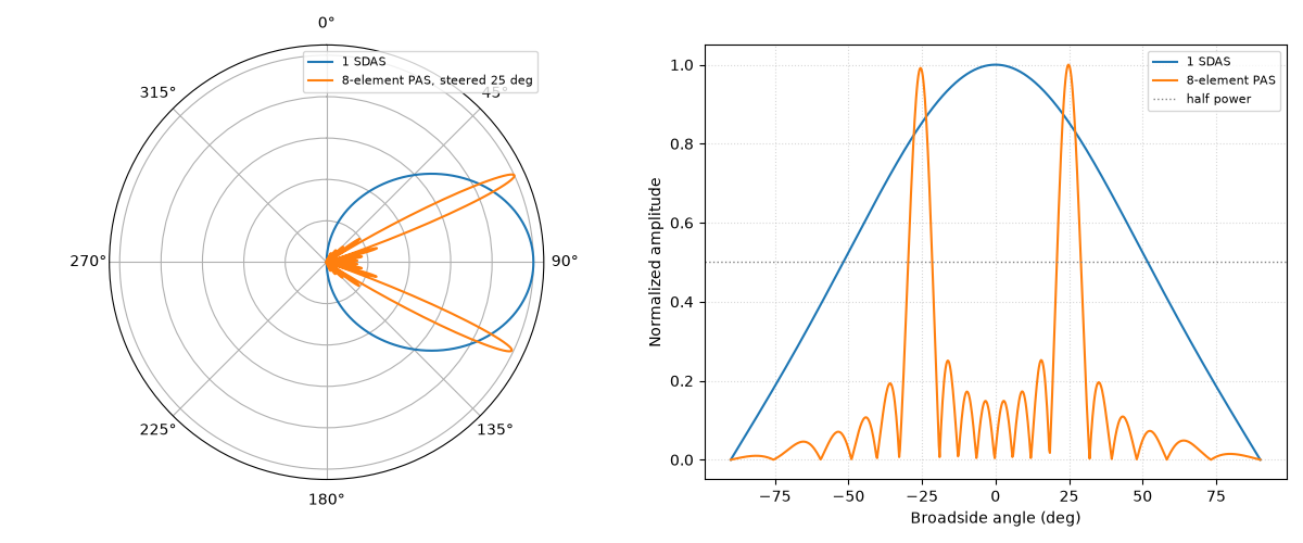
A concrete design choice: an 8-element array, 2 km spacing, at the 1024 Hz upper CSAMT frequency, steered 25 degrees off broadside — the full combined pattern plus its quantitative payoff over one plain SDAS transmitter.

N_design = 8
beta_25 = beam_steer(25.0, d, k_hf)
pattern_design = pas_pattern(
    theta_b, N=N_design, d=d, k=k_hf, beta=beta_25, l=1000.0
)
pattern_single = sdas_element_pattern(
    90.0 - np.abs(theta_b), l=1000.0, k=k_hf
)

fig = plt.figure(figsize=(12.0, 5.0))
axp = fig.add_subplot(1, 2, 1, projection="polar")
axc = fig.add_subplot(1, 2, 2)
plot_radiation_pattern(
    theta_b,
    [pattern_single, pattern_design],
    labels=["1 SDAS", f"{N_design}-element PAS, steered 25 deg"],
    ax=axp,
    title="",
)
# Isolate the *main* lobe's own half-power width — the crude global
# span of all points >= 0.5 also catches the section-4 grating lobe on
# the other side of broadside, overstating the width several-fold.
above_half = pattern_design >= 0.5
peak_idx = int(np.argmax(pattern_design))
lo = peak_idx
while lo > 0 and above_half[lo - 1]:
    lo -= 1
hi = peak_idx
while hi < above_half.size - 1 and above_half[hi + 1]:
    hi += 1
beamwidth = float(theta_b[hi] - theta_b[lo])
axc.plot(theta_b, pattern_single, label="1 SDAS")
axc.plot(theta_b, pattern_design, label=f"{N_design}-element PAS")
axc.axhline(0.5, color="0.5", ls=":", lw=1, label="half power")
axc.set_xlabel("Broadside angle (deg)")
axc.set_ylabel("Normalized amplitude")
axc.legend(fontsize=8)
axc.grid(True, ls=":", alpha=0.5)
fig.tight_layout()

print(
    f"{N_design}-element array SNR gain over 1 SDAS: {snr_gain_db(N_design):.1f} dB"
)
print(f"steered main-lobe half-power width: {beamwidth:.1f} deg")

8-element array SNR gain over 1 SDAS: 18.1 dB
steered main-lobe half-power width: 8.0 deg

Reading this figure/output. The 8-element design’s main lobe (right panel, orange) is dramatically narrower than the single-SDAS element pattern (blue) and is clearly pointed toward 25°, not broadside — visible confirmation that steering and array narrowing combine as intended. Quantitatively, this design buys an 18.1 dB SNR improvement over one plain transmitter, concentrated into a main lobe only about 8 degrees wide at half power. The bump near -25° is not a minor side effect, either: at amplitude 0.99 versus the main lobe’s 1.00, it is essentially the same strength — the grating lobe already found in section 4 for this spacing/frequency combination, now shown to carry almost exactly as much energy as the intended beam. This design’s SNR gain is not obtained for free: at 1024 Hz, nearly half of it is being radiated toward -25° instead of the intended +25° area of interest.