1-D MT, CSAMT and TEM soundings

Given a layered model (see 1-D layered models and geology priors), the 1-D solvers compute what an instrument would actually record. MT1DForward and CSAMT1DForward return apparent resistivity and phase versus frequency; TEM1DForward returns a transient decay versus time. This example runs all three, and shows the standard ways to visualise a sounding: the two-panel resistivity/phase curve, the three-panel “model + response” validation view, and a multi-model comparison.

Models and frequency bands

We reuse the model library from the previous example and define the frequency/time grids each method samples: a broad MT/AMT band, a narrower CSAMT band (10 Hz - 10 kHz), and a set of TEM gate times.

import matplotlib.pyplot as plt
import numpy as np

from pycsamt.api.control import PYCSAMT_CONTROL
from pycsamt.api.style import PYCSAMT_STYLE
from pycsamt.forward import (
    CSAMT1DForward,
    LayeredModel,
    MT1DForward,
    TEM1DForward,
    plot_response_1d,
    plot_response_and_model_1d,
)

# Use the multi-model comparison (5th figure) as the gallery thumbnail.

M_SEDIMENTARY = LayeredModel(
    [1_000.0, 20.0, 5.0, 300.0], [200.0, 600.0, 1_500.0], name="sedimentary"
)
M_CRYSTALLINE = LayeredModel(
    [800.0, 8_000.0, 600.0], [2_000.0, 15_000.0], name="crystalline"
)
M_GEOTHERMAL = LayeredModel(
    [500.0, 8.0, 250.0, 3_000.0], [100.0, 400.0, 2_500.0], name="geothermal"
)
M_CONDUCTIVE = LayeredModel(
    [200.0, 5.0, 400.0, 100.0],
    [150.0, 500.0, 2_000.0],
    name="conductive-layer",
)
M_HALFSPACE = LayeredModel([100.0], [], name="halfspace")

FREQS_MT = np.logspace(-3, 4, 35)  # broad MT/AMT band
FREQS_CSAMT = np.logspace(1, 4, 25)  # CSAMT: 10 Hz - 10 kHz
TIMES_TEM = np.logspace(-6, -2, 30)  # TEM gate times

# Run the MT forward on every model once; reuse the responses below.
R_SED = MT1DForward(FREQS_MT).run(M_SEDIMENTARY)
R_CRYS = MT1DForward(FREQS_MT).run(M_CRYSTALLINE)
R_GEO = MT1DForward(FREQS_MT).run(M_GEOTHERMAL)
R_COND = MT1DForward(FREQS_MT).run(M_CONDUCTIVE)
R_HS = MT1DForward(FREQS_MT).run(M_HALFSPACE)

1. The classic two-panel sounding

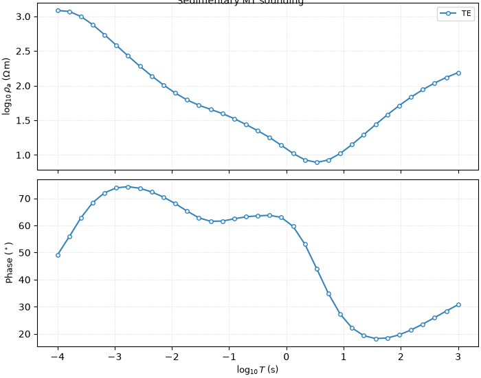
plot_response_1d() draws apparent resistivity (top) and phase (bottom) against period. For the sedimentary model the conductive middle section pulls the mid-period apparent resistivity down and drives the phase above 45 degrees.

axs = plot_response_1d(R_SED, title="Sedimentary MT sounding")

2. A different model, a different signature

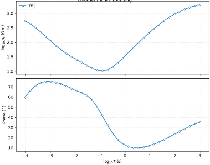
The geothermal model’s shallow conductive clay cap produces a deep apparent-resistivity minimum and a stronger phase excursion — the textbook response geothermal MT surveys look for.

axs = plot_response_1d(R_GEO, title="Geothermal MT sounding")

3. Model and response together: the validation view

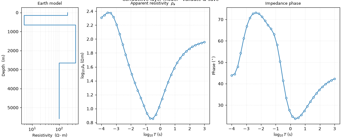
plot_response_and_model_1d() places the resistivity-depth model beside its apparent-resistivity and phase response — the single most useful figure when checking that a forward run behaves as expected before trusting it downstream.

fig = plot_response_and_model_1d(
    R_COND,
    M_CONDUCTIVE,
    title="Conductive-layer model - validate & save",
    figsize=(11, 4.5),
)

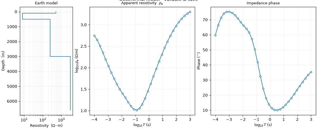
The same view for the geothermal model makes the link between the shallow conductor and the response minimum explicit:

fig = plot_response_and_model_1d(
    R_GEO,
    M_GEOTHERMAL,
    title="Geothermal model - validate & save",
    figsize=(11, 4.5),
)

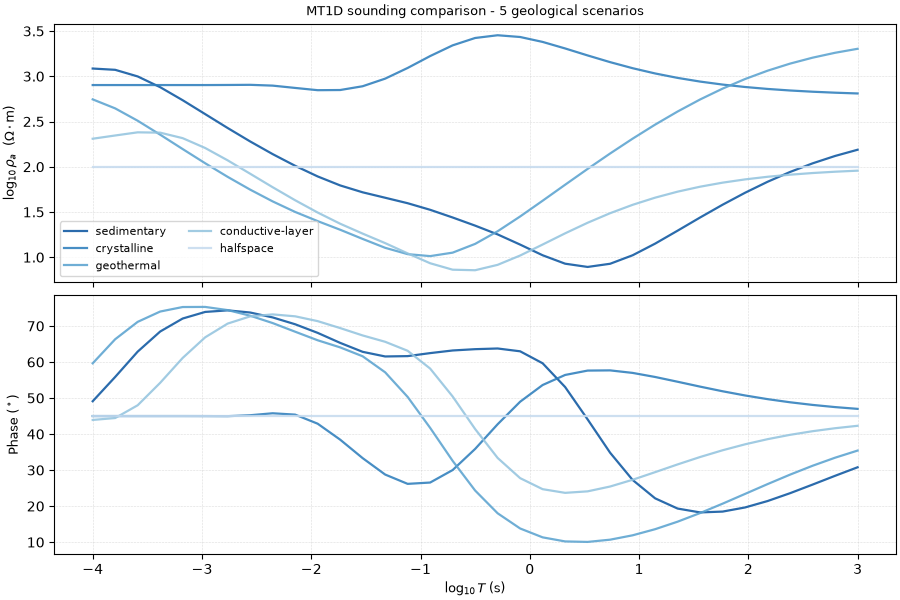
4. Comparing several soundings at once

There is no single “overlay” helper, but the response objects expose rho_a and phase arrays directly, so a comparison plot is a few lines. We use the library’s own multiline colour cycle (PYCSAMT_STYLE) and its period-axis transform (PYCSAMT_CONTROL) so the styling matches every other figure.

fig, axs = plt.subplots(
    2, 1, figsize=(9, 6), sharex=True, constrained_layout=True
)
responses = [R_SED, R_CRYS, R_GEO, R_COND, R_HS]
labels = [
    "sedimentary",
    "crystalline",
    "geothermal",
    "conductive-layer",
    "halfspace",
]
colors = PYCSAMT_STYLE.multiline.colors(5)
x = PYCSAMT_CONTROL.x.transform(FREQS_MT)
for k, (resp, lab) in enumerate(zip(responses, labels)):
    kw = dict(color=colors[k], lw=1.6, alpha=0.88, label=lab)
    axs[0].plot(x, np.log10(resp.rho_a), **kw)
    axs[1].plot(x, resp.phase, **kw)
for ax in axs:
    ax.grid(True, which="both", ls=":", lw=0.4, color="0.75")
    ax.set_axisbelow(True)
axs[0].set_ylabel(r"$\log_{10}\rho_a$  ($\Omega\cdot$m)", fontsize=9)
axs[1].set_ylabel(r"Phase ($^\circ$)", fontsize=9)
axs[1].set_xlabel(PYCSAMT_CONTROL.x.label(), fontsize=9)
axs[0].legend(fontsize=8, ncol=2, framealpha=0.8)
axs[0].set_title(
    "MT1D sounding comparison - 5 geological scenarios", fontsize=9
)

Text(0.5, 1.0, 'MT1D sounding comparison - 5 geological scenarios')

5. The CSAMT sounding

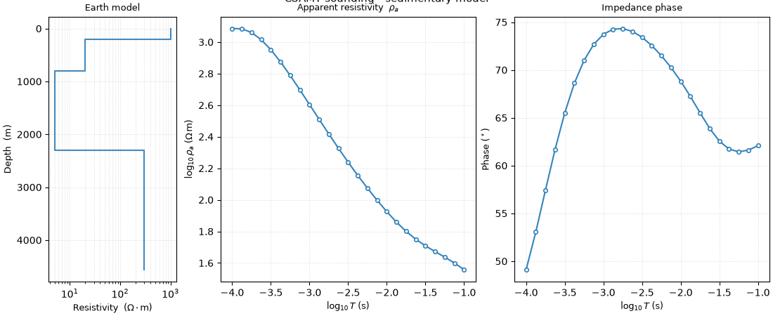
CSAMT1DForward uses the same model but the CSAMT band, and is validated the same way. Over 10 Hz - 10 kHz only the shallow part of the sedimentary section is resolved, so the response probes a shallower depth range than the broadband MT sounding above.

R_SED_CSAMT = CSAMT1DForward(FREQS_CSAMT).run(M_SEDIMENTARY)
fig = plot_response_and_model_1d(
    R_SED_CSAMT,
    M_SEDIMENTARY,
    title="CSAMT sounding - sedimentary model",
    figsize=(11, 4.5),
)

6. The TEM transient

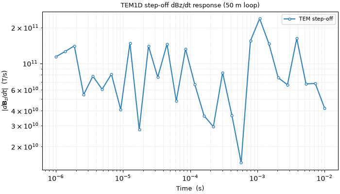
TEM1DForward models a transient (time-domain) step-off: after the transmitter current is cut, it returns the decaying vertical-field rate dBz/dt at each gate time rather than an apparent resistivity. We plot the decay directly on log-log axes.

R_TEM = TEM1DForward(TIMES_TEM, loop_radius=50.0).run(M_CONDUCTIVE)
fig, ax = plt.subplots(figsize=(7, 4), constrained_layout=True)
ax.loglog(
    R_TEM.times,
    np.abs(R_TEM.dBz_dt),
    color=PYCSAMT_STYLE.mt.te.color,
    lw=1.6,
    marker="o",
    ms=3.5,
    mfc="white",
    mew=1.0,
    alpha=0.9,
    label="TEM step-off",
)
ax.set_xlabel("Time  (s)", fontsize=9)
ax.set_ylabel(r"$|d\mathbf{B}_z/dt|$  (T/s)", fontsize=9)
ax.set_title("TEM1D step-off dBz/dt response (50 m loop)", fontsize=9, pad=6)
ax.legend(fontsize=8)
ax.grid(True, which="both", ls=":", lw=0.4, color="0.75")
ax.set_axisbelow(True)