Quasi-3-D forward modelling

Grid3D and MT3DForward extend the workflow to a full 3-D resistivity volume, returning the complete impedance tensor on a station grid. This example builds a uniform half-space (a validation baseline) and a conductive block embedded in a resistive background, then walks through the 3-D viewers: model slices, map views, pseudo-sections, and full-tensor component panels.

Two 3-D models

Grid3D.halfspace gives a uniform reference volume; Grid3D.block_anomaly embeds a 5 Ohm-m block in a 500 Ohm-m host. Both use a 4x4 station grid over a padded 8x8x6 mesh, and the forward runs over 1 Hz - 1 kHz.

import numpy as np

from pycsamt.forward import (
    Grid3D,
    MT3DForward,
    plot_model_3d,
    plot_response_map_3d,
    plot_response_section_3d,
    plot_tensor_components_3d,
)

# Use the full-tensor apparent-resistivity panel (9th figure) as thumbnail.

FREQS_3D = np.logspace(0, 3, 12)  # 1 Hz - 1 kHz

G3_HALF = Grid3D.halfspace(
    rho=100.0,
    nx=8,
    ny=8,
    nz=6,
    x_max=4_000.0,
    y_max=4_000.0,
    z_max=2_000.0,
    n_pad=3,
    nx_stations=4,
    ny_stations=4,
    name="halfspace-3D",
)
G3_BLOCK = Grid3D.block_anomaly(
    bg_rho=500.0,
    anomaly_rho=5.0,
    bounds=(1_200.0, 2_800.0, 1_200.0, 2_800.0, 300.0, 1_200.0),
    nx=8,
    ny=8,
    nz=6,
    x_max=4_000.0,
    y_max=4_000.0,
    z_max=2_000.0,
    n_pad=3,
    nx_stations=4,
    ny_stations=4,
    name="block-anomaly-3D",
)

1. Model slices

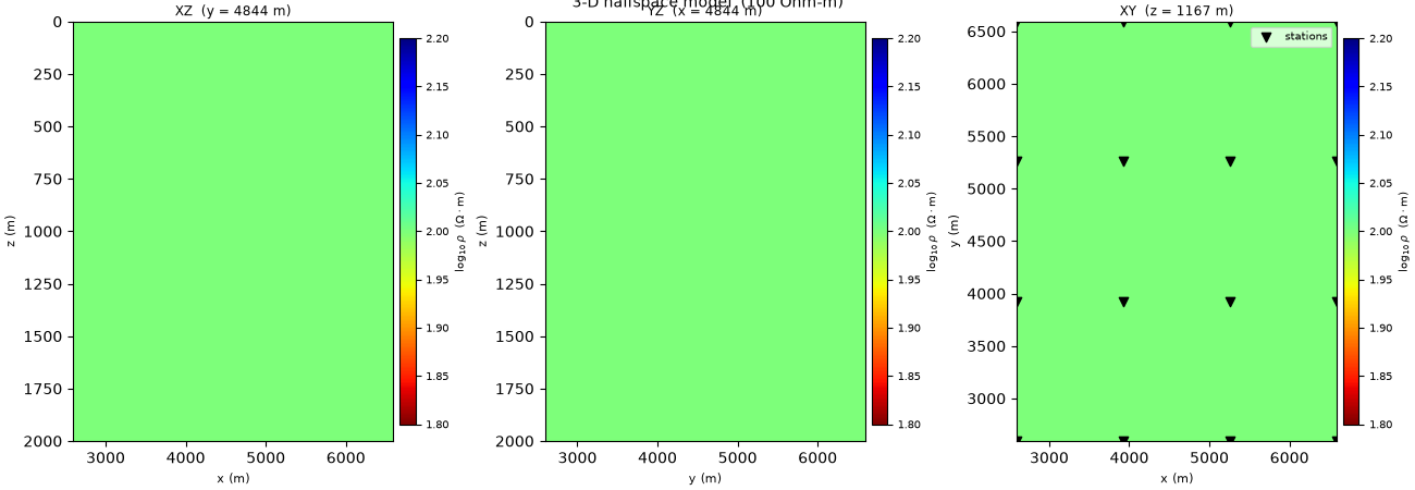
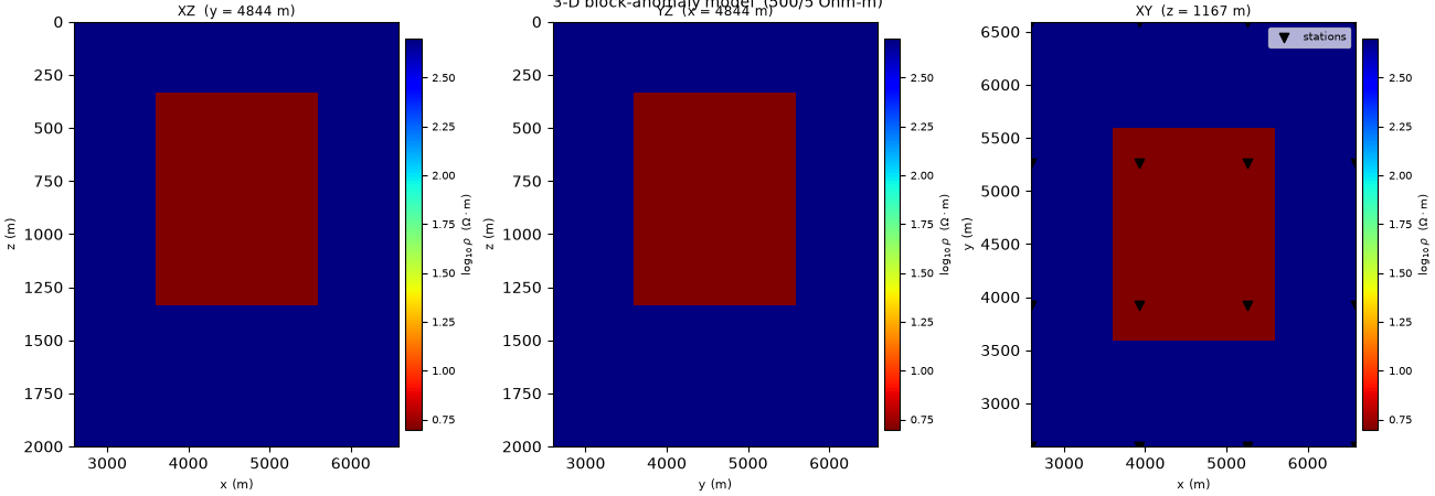
plot_model_3d() shows orthogonal slices through the volume. The half-space is uniform by construction — a useful sanity check that the mesh and station layout are what you intended.

fig = plot_model_3d(G3_HALF, title="3-D halfspace model  (100 Ohm-m)")

The block-anomaly model makes the conductive target visible in the depth and plan slices:

fig = plot_model_3d(G3_BLOCK, title="3-D block-anomaly model  (500/5 Ohm-m)")

Run the quasi-3-D forward on both models.

R3_HALF = MT3DForward(FREQS_3D, G3_HALF, verbose=False).run()
R3_BLOCK = MT3DForward(FREQS_3D, G3_BLOCK, verbose=False).run()

2. Map views

plot_response_map_3d() images one quantity across the station grid at a single frequency. The half-space returns a flat, uniform apparent-resistivity map (the expected baseline):

ax = plot_response_map_3d(
    R3_HALF,
    freq_idx=0,
    component="xy",
    title=r"Halfspace - map $\rho_a$ [Z_XY] (T = 1 s)",
)

Over the block anomaly, the same map shows the conductor’s footprint pulling apparent resistivity down near the model centre:

ax = plot_response_map_3d(
    R3_BLOCK,
    freq_idx=4,
    component="xy",
    title=r"Block anomaly - map $\rho_a$ [Z_XY]",
)

Phase responds to the same structure with opposite polarity:

ax = plot_response_map_3d(
    R3_BLOCK,
    freq_idx=4,
    component="xy",
    quantity="phase",
    title=r"Block anomaly - map phase [Z_XY]",
)

3. Pseudo-sections

plot_response_section_3d() extracts a station-vs-period section through the 3-D response — the 3-D analogue of the 2-D pseudo-sections. Half-space first (flat baseline):

ax = plot_response_section_3d(
    R3_HALF,
    component="xy",
    title=r"Halfspace - 3-D pseudo-section $\rho_a$ [Z_XY]",
)

The block anomaly imprints a closed low-resistivity zone; n_contours overlays isolines:

ax = plot_response_section_3d(
    R3_BLOCK,
    component="xy",
    n_contours=4,
    title=r"Block anomaly - 3-D pseudo-section $\rho_a$ [Z_XY]",
)

The cross-component yx phase section highlights the same target from the orthogonal polarisation:

ax = plot_response_section_3d(
    R3_BLOCK,
    component="yx",
    quantity="phase",
    title=r"Block anomaly - pseudo-section phase [Z_YX]",
)

4. Full impedance-tensor panels

plot_tensor_components_3d() lays out all four tensor elements (XX, XY, YX, YY) as a 2x2 map panel at one frequency — the most complete single view of a quasi-3-D response. The off-diagonal (XY, YX) maps carry the main anomaly signal; the diagonal (XX, YY) maps reveal the 3-D coupling a 1-D or 2-D model cannot produce.

ax = plot_tensor_components_3d(
    R3_BLOCK,
    freq_idx=4,
    title=r"Block anomaly - full impedance tensor $\rho_a$",
)

The same panel as phase:

ax = plot_tensor_components_3d(
    R3_BLOCK,
    freq_idx=4,
    quantity="phase",
    title="Block anomaly - full impedance tensor phase",
)