Calibration against boreholes

An inverted resistivity model is only as good as its tie to ground truth. ModelCalibrator adjusts the model so its resistivity-to-lithology mapping honours borehole logs, and reports how much each station had to move. This example calibrates the synthetic section against two boreholes and compares before and after.

Boreholes and the native model

The two boreholes log the true four-unit sequence at 500 m and 1500 m. Borehole holds a list of depth Interval s with lithology labels.

from _interp_data import demo_boreholes, demo_model

from pycsamt.interp import ModelCalibrator

# Use the before/after calibrated-model panel (1st figure) as the thumbnail.

rm = demo_model()
boreholes = demo_boreholes()
for bh in boreholes:
    print(
        f"{bh.name} @ x={bh.x:.0f} m: "
        f"{', '.join(iv.lithology for iv in bh.intervals)}"
    )

BH-1 @ x=500 m: overburden, sand aquifer, clay, granite basement
BH-2 @ x=1500 m: overburden, sand aquifer, clay, granite basement

Calibrate

ModelCalibrator.fit compares each near-borehole sounding to the log and rescales the model’s resistivity-lithology boundaries to match, returning a corrected ResistivityModel via calibrated_model().

cal = ModelCalibrator(max_borehole_distance=800.0, verbose=False).fit(
    rm, boreholes
)
nm = cal.calibrated_model()
print("native method:", rm.method)
print("calibrated method:", nm.method)

native method: synthetic
calibrated method: synthetic+calibrated

Before and after

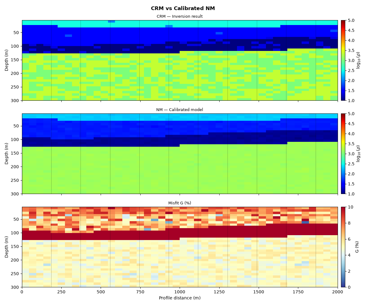
PlotCalibratedModel stacks the native model, the calibrated model, and their difference, with the borehole positions marked — so you can see exactly where and how much the calibration moved the resistivities.

from pycsamt.interp.plot import PlotCalibratedModel

PlotCalibratedModel(nm, rm).plot()

<Figure size 1200x1000 with 6 Axes>

Reading it. The difference panel is near-zero away from the boreholes and picks up where the model’s unit boundaries were nudged to match the logs. On real data, large corrections concentrated near a borehole warn that the inversion mis-placed a boundary there — worth revisiting before the model feeds hydro-geophysics.