Time-lapse monitoring

Repeat EM surveys track how the subsurface changes — a rising water table, a spreading plume, managed recharge. TimeLapseEM holds a baseline model plus one or more monitor surveys on the same grid and differences them, and the plot classes turn those differences into monitoring figures. This example simulates a wetting front with three surveys of the synthetic section.

Build the time series

We reuse the shared model with an increasing wet factor, which lowers the aquifer resistivity as pore water increases — a stand-in for three repeat surveys over a wetting aquifer.

from _interp_data import demo_model

from pycsamt.interp import (
    TimeLapseEM,
    assert_compatible_grids,
)

# Use the difference section (1st figure) as the card thumbnail.

surveys = [
    demo_model(wet=1.0, seed=1),
    demo_model(wet=1.6, seed=2),
    demo_model(wet=2.4, seed=3),
]
assert_compatible_grids(surveys)  # same grid is required to difference
tl = TimeLapseEM(surveys, labels=["baseline", "month 1", "month 2"])
print("surveys:", tl.labels)

surveys: ['baseline', 'month 1', 'month 2']

The difference section

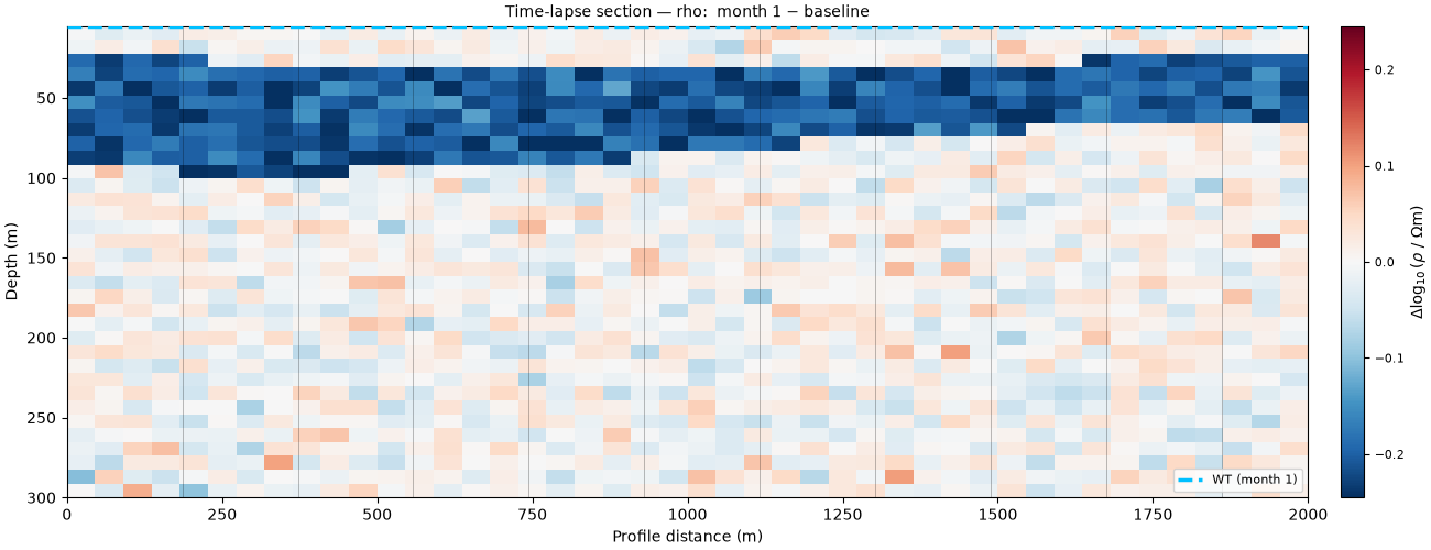
PlotTimeLapseSection images \(\Delta\log_{10}\rho\) between a chosen survey and the baseline. A coherent negative anomaly (resistivity dropping) traces where water has been added since the baseline.

from pycsamt.interp.plot import (
    PlotMultiTimeLapseGrid,
    PlotTimeLapseSection,
)

PlotTimeLapseSection(tl, quantity="rho").plot()

<Figure size 1300x500 with 2 Axes>

All surveys at a glance

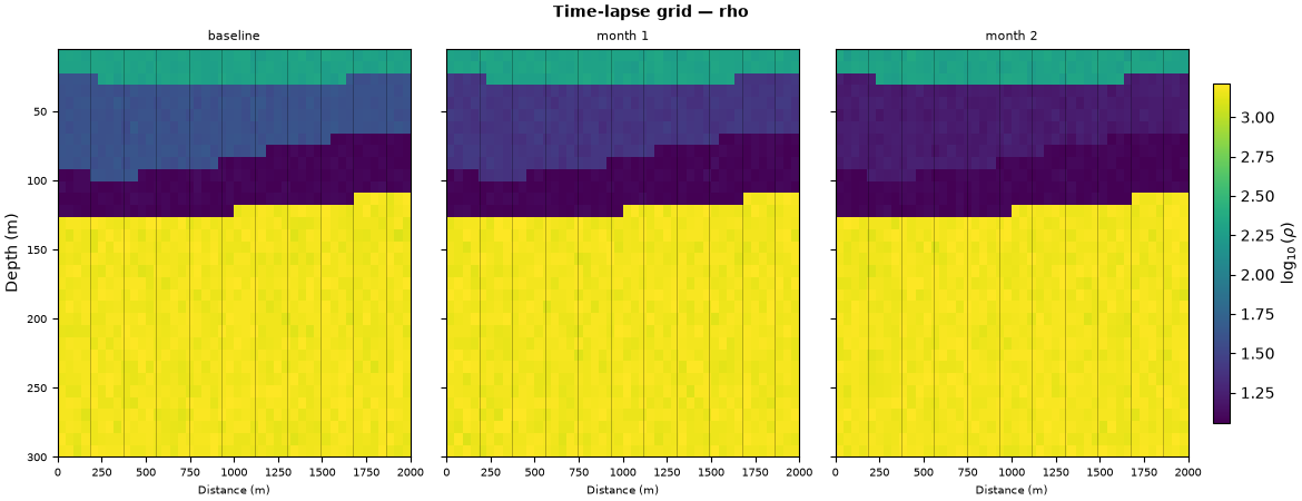
PlotMultiTimeLapseGrid lays the surveys out in a row under one shared colour scale, so the progression of the change reads left to right — the standard monitoring montage.

PlotMultiTimeLapseGrid(tl).plot()

<Figure size 1170x450 with 4 Axes>

Reading it. The difference section localises the change to the aquifer interval, and the grid shows it strengthening survey to survey — exactly the wetting front built into the models. On real monitoring data, always check that changes sit inside known hydrogeological units (here the aquifer) and not at the surface or edges, where they usually mean acquisition or static-shift drift rather than real subsurface change.