Controlled-source edge QC on a real Zonge CSAMT sounding

Natural-source AMT/MT QC assumes a plane-wave field. CSAMT does not: an operator drives a grounded dipole, and the field questions change to is the receiver in the far field, is the transmitter current steady, and is there energy at every transmitted frequency? This example runs the pycsamt.iot controlled-source edge diagnostics on a real Zonge CSAMT average file (data/avg/K1.AVG): 47 station-positions, the classic 0.125 - 8192 Hz transmitter comb, and the injected current logged with every reading.

The workflow is:

1. load the real .avg sounding (frequency, apparent resistivity, phase, and transmitter current per reading);

2. classify each frequency into near / transition / far field from the skin depth versus the transmitter-receiver offset – the core CSAMT QC;

3. assess transmitter-current stability from the logged amps; and

4. confirm the acquisition frequency comb matches the CSAMT method profile.

1. Load the real CSAMT sounding

load_avg returns a tidy per-reading table. We take one representative station-position along the line; the transmitter comb and injected current come straight from the file.

from __future__ import annotations

import os
import warnings
from pathlib import Path

import matplotlib.pyplot as plt
import numpy as np
import pandas as pd

from pycsamt.iot import (
    assess_source_stability,
    classify_field_zones,
    method_profile,
    skin_depth_m,
    target_bands_for_method,
)

warnings.filterwarnings("ignore")

Z_NEAR, Z_TRANS, Z_FAR = "#D55E00", "#E69F00", "#009E73"  # near/trans/far
ZONE_COLOR = {"near": Z_NEAR, "transition": Z_TRANS, "far": Z_FAR}
CURRENT = "#0072B2"

# A representative transmitter-receiver offset for this survey. The exact
# value comes from the field geometry; the field-zone verdict scales with it.
TX_RX_OFFSET_M = 5000.0


def style_axis(ax: plt.Axes) -> None:
    ax.spines["top"].set_visible(False)
    ax.spines["right"].set_visible(False)
    ax.grid(True, which="both", color="#000000", alpha=0.07, lw=0.7)
    ax.set_axisbelow(True)


def repo_root() -> Path:
    env_root = os.environ.get("PYCSAMT_DOCS_REPO_ROOT")
    if env_root:
        return Path(env_root)
    return Path(__file__).resolve().parents[3]


def _synthetic_avg() -> pd.DataFrame:
    """A CSAMT-plausible stand-in when the bundled .avg is absent."""
    freq = np.array(
        [
            0.125,
            0.25,
            0.5,
            1,
            2,
            4,
            8,
            16,
            32,
            64,
            128,
            256,
            512,
            1024,
            2048,
            4096,
            8192.0,
        ]
    )
    # far-field rho ~ 300 ohm.m; near-field low-freq rise; keyed current.
    rho = 300.0 * (1.0 + 40.0 / (freq + 0.2))
    phase = 45.0 - 10.0 * np.log10(freq / freq.min() + 1)
    amps = np.clip(9.5 - 6.0 * (freq < 1.0), 3.5, 10.0)
    return pd.DataFrame(
        {
            "station": "SYNTH",
            "freq": freq,
            "rho": rho,
            "phase": phase,
            "amps": amps,
        }
    )


avg_path = repo_root() / "data" / "avg" / "K1.AVG"
if avg_path.is_file():
    from pycsamt.zonge import load_avg

    df, _meta = load_avg(str(avg_path))
    for col in ("freq", "rho", "phase", "amps"):
        df[col] = pd.to_numeric(df[col], errors="coerce")
    source = avg_path.name
else:  # pragma: no cover - clean checkout without the bundled file
    print("NOTE: bundled K1.AVG absent - using a synthetic CSAMT stand-in.")
    df = _synthetic_avg()
    source = "synthetic"

# a mid-line station with a full frequency sweep
counts = df.groupby("station")["freq"].nunique()
station = counts.sort_values().index[len(counts) // 2]
sub = (
    df[df["station"] == station]
    .dropna(subset=["freq", "rho"])
    .sort_values("freq")
)
freq = sub["freq"].to_numpy(float)
rho = sub["rho"].to_numpy(float)
amps = sub["amps"].to_numpy(float)
print(f"source={source}  station-position={station}  n_freq={len(freq)}")
print(f"frequency comb: {freq.min():g} - {freq.max():g} Hz")
print(
    f"apparent resistivity: {np.nanmin(rho):.0f} - {np.nanmax(rho):.0f} ohm.m"
)
print(f"transmitter current: {np.nanmin(amps):.1f} - {np.nanmax(amps):.1f} A")

source=K1.AVG  station-position=2050.0  n_freq=17
frequency comb: 0.125 - 8192 Hz
apparent resistivity: 15 - 25871 ohm.m
transmitter current: 5.0 - 10.0 A

2. Field zones from skin depth vs offset

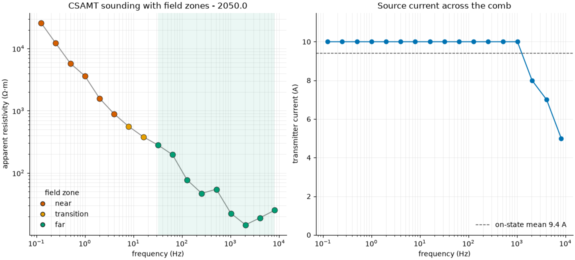
The far-field (plane-wave) assumption only holds when the receiver is many skin depths from the source. At low frequency the skin depth grows past the transmitter-receiver offset and the sounding rolls into the transition and near field, where CSAMT apparent resistivities must not be read as plane-wave values.

zones = classify_field_zones(freq, rho, offset_m=TX_RX_OFFSET_M)
delta = skin_depth_m(rho, freq)
first_far = zones.first_far_field_hz()
print(
    f"field zones: {zones.n_near} near, {zones.n_transition} transition, "
    f"{zones.n_far} far"
)
print(
    f"far-field fraction: {zones.far_fraction:.0%}  "
    f"(plane-wave valid at >= {first_far:g} Hz)"
    if first_far
    else "far-field fraction: none reached"
)
print(f"near-field correction recommended: {zones.correction_recommended}")

field zones: 6 near, 2 transition, 9 far
far-field fraction: 53%  (plane-wave valid at >= 32 Hz)
near-field correction recommended: True

3. Transmitter-current stability

The injected current sets the signal level of every reading, so its steadiness bounds data quality. The real log shows the current dropping at the low frequencies (a common CSAMT limitation), which assess_source_stability picks up.

source_status = assess_source_stability(amps, max_cv=0.1)
print(
    f"source stable: {source_status.stable}  "
    f"(current CV={source_status.current_cv:.3f}, "
    f"mean={source_status.current_mean_a:.1f} A)"
)
if source_status.flags:
    print(f"source flags: {source_status.flags}")

source stable: False  (current CV=0.146, mean=9.4 A)
source flags: ['current_unstable']

4. Frequency comb vs the CSAMT method profile

CSAMT transmits a discrete set of frequencies. The recorded comb should span the method’s expected band – and here the real 0.125 - 8192 Hz comb matches the CSAMT profile exactly.

profile = method_profile("csamt")
band = profile.frequency_band_hz
in_band = int(np.sum((freq >= band[0]) & (freq <= band[1])))
print(f"CSAMT profile band: {band[0]} - {band[1]} Hz")
print(f"comb lines in band: {in_band}/{len(freq)}")
print(f"target sub-bands: {target_bands_for_method('csamt')}")

CSAMT profile band: 0.125 - 8192.0 Hz
comb lines in band: 17/17
target sub-bands: [(0.125, 1.0), (1.0, 10.0), (10.0, 100.0), (100.0, 1000.0), (1000.0, 8192.0)]

5. The controlled-source QC picture

Left: the apparent-resistivity sounding, each frequency coloured by its field zone, with the plane-wave-valid band shaded. Right: the transmitter current across the comb, with the on-state mean marked. The low-frequency near-field rise and the coincident current drop are exactly the operational faults controlled-source edge QC exists to catch.

zone_colours = [ZONE_COLOR[z] for z in zones.zones]

fig, (ax_rho, ax_cur) = plt.subplots(
    1,
    2,
    figsize=(11.5, 5.2),
    constrained_layout=True,
)

good = np.isfinite(rho) & (rho > 0)
ax_rho.loglog(freq[good], rho[good], "-", color="#888", lw=1.2, zorder=1)
for f, r, c in zip(freq[good], rho[good], np.array(zone_colours)[good]):
    ax_rho.loglog([f], [r], "o", ms=8, color=c, mec="#222", mew=0.6, zorder=3)
if first_far:
    ax_rho.axvspan(first_far, freq.max(), color=Z_FAR, alpha=0.08, lw=0)
ax_rho.set(
    xlabel="frequency (Hz)",
    ylabel=r"apparent resistivity ($\Omega\!\cdot\!$m)",
    title=f"CSAMT sounding with field zones - {station}",
)
handles = [
    plt.Line2D(
        [], [], marker="o", ls="", mec="#222", color=ZONE_COLOR[z], label=z
    )
    for z in ("near", "transition", "far")
]
ax_rho.legend(handles=handles, frameon=False, title="field zone")
style_axis(ax_rho)

ax_cur.semilogx(freq, amps, "o-", color=CURRENT, ms=6, lw=1.4)
ax_cur.axhline(
    source_status.current_mean_a,
    color="#444",
    ls="--",
    lw=1.0,
    label=f"on-state mean {source_status.current_mean_a:.1f} A",
)
ax_cur.set(
    xlabel="frequency (Hz)",
    ylabel="transmitter current (A)",
    title="Source current across the comb",
    ylim=(0, max(11.0, np.nanmax(amps) * 1.15)),
)
ax_cur.legend(frameon=False, loc="lower right")
style_axis(ax_cur)

plt.show()