Edge QC on a real long-period MT recording

This example runs the pycsamt.iot edge-QC layer on a real field recording: the bundled SAMTEX/LiMS long-period magnetotelluric series data/MT/TS/kap103as.ts (station kap103, five channels, 5 s sampling, ~27 days). Real recordings are imperfect — this one carries genuine data gaps — so it is an honest test of what an IoT recorder would flag at the edge before the series is turned into cross-spectra and an EDI file.

Because the series is long-period (0.2 Hz sampling, 0.1 Hz Nyquist), the mains-harmonic detector does not apply here; the diagnostics that matter for this band are sensor dropout, data coverage, SNR, and the resolvable frequency band. The same edge result is then turned into a telemetry packet and given a reproducible provenance record.

1. Load the real MT time series

pycsamt.ts.read_ts reads the LiMS .ts container into a TSData object with per-channel arrays (missing samples are NaN), the sampling interval, and station coordinates.

from __future__ import annotations

import tempfile
from pathlib import Path

import matplotlib.pyplot as plt
import numpy as np
from _ts_sample import load_ts_sample, real_ts_path

from pycsamt.iot import (
    DeviceConfig,
    EdgeProcessingConfig,
    EdgeProcessor,
    FieldSession,
    ProvenanceRecord,
    build_acquisition_manifest,
    compute_live_spectra,
    detect_sensor_dropout,
    estimate_channel_snr,
    estimate_frequency_coverage,
    export_reproducibility_bundle,
)

# Okabe-Ito, a colour-blind-safe categorical palette. Magnetic channels get
# cool hues, electric channels warm ones, assigned in a fixed order.
CH_COLORS = {
    "hx": "#0072B2",
    "hy": "#56B4E9",
    "hz": "#009E73",
    "ex": "#D55E00",
    "ey": "#E69F00",
}
STATUS = {"ok": "#009E73", "warn": "#E69F00", "bad": "#D55E00"}


def style_axis(ax: plt.Axes) -> None:
    """Recessive axes: drop top/right spines, add a light y grid."""
    ax.spines["top"].set_visible(False)
    ax.spines["right"].set_visible(False)
    ax.grid(True, axis="y", color="#000000", alpha=0.08, lw=0.8)
    ax.set_axisbelow(True)


ts_path = real_ts_path()
record, ts_is_real = load_ts_sample()
if not ts_is_real:
    print("NOTE: bundled TS recording absent — using a synthetic sample.")

channels = [c.lower() for c in record.channels()]
sample_rate = 1.0 / float(record.dt)
duration_days = record.n_samples * record.dt / 86400.0
data = {c: np.asarray(record.get(c.upper()), dtype=float) for c in channels}

print(
    f"station={record.station}  dt={record.dt:g}s  fs={sample_rate:g} Hz  "
    f"channels={channels}\n"
    f"n_samples={record.n_samples:,}  (~{duration_days:.1f} days)  "
    f"lat={record.lat:.4f}  lon={record.lon:.4f}"
)

NOTE: bundled TS recording absent — using a synthetic sample.
station=kap103-synthetic  dt=5s  fs=0.2 Hz  channels=['hx', 'hy', 'hz', 'ex', 'ey']
n_samples=65,536  (~3.8 days)  lat=-32.1389  lon=20.4675

2. Edge diagnostics per channel

For each channel we quantify data coverage and dropouts, a time-domain SNR proxy, and the resolvable frequency band. These are exactly the scalars an edge node would stream as a QC packet.

rows = []
for channel in channels:
    signal = data[channel]
    dropout = detect_sensor_dropout(signal, min_flat_run=20)
    coverage = 1.0 - dropout["nan_fraction"]
    band = estimate_frequency_coverage(signal, sample_rate)
    rows.append(
        {
            "channel": channel,
            "coverage_%": 100.0 * coverage,
            "n_nan": dropout["n_nan"],
            "longest_flat_run": dropout["longest_flat_run"],
            "snr_db": estimate_channel_snr(signal, sample_rate),
            "f_low_mHz": 1e3 * band.f_low_hz,
            "f_high_mHz": 1e3 * band.f_high_hz,
        }
    )

try:
    import pandas as pd

    print(
        pd.DataFrame(rows).to_string(
            index=False, float_format=lambda v: f"{v:.3f}"
        )
    )
except Exception:  # pragma: no cover - pandas always present in docs
    for row in rows:
        print(row)

channel  coverage_%  n_nan  longest_flat_run  snr_db  f_low_mHz  f_high_mHz
     hx     100.000      0                 1  39.931      0.781      22.656
     hy     100.000      0                 1  45.430      0.781      22.656
     hz     100.000      0                 1  41.709      0.781      21.875
     ex     100.000      0                 1  45.436      0.781      22.656
     ey     100.000      0                 1  39.901      0.781      22.656

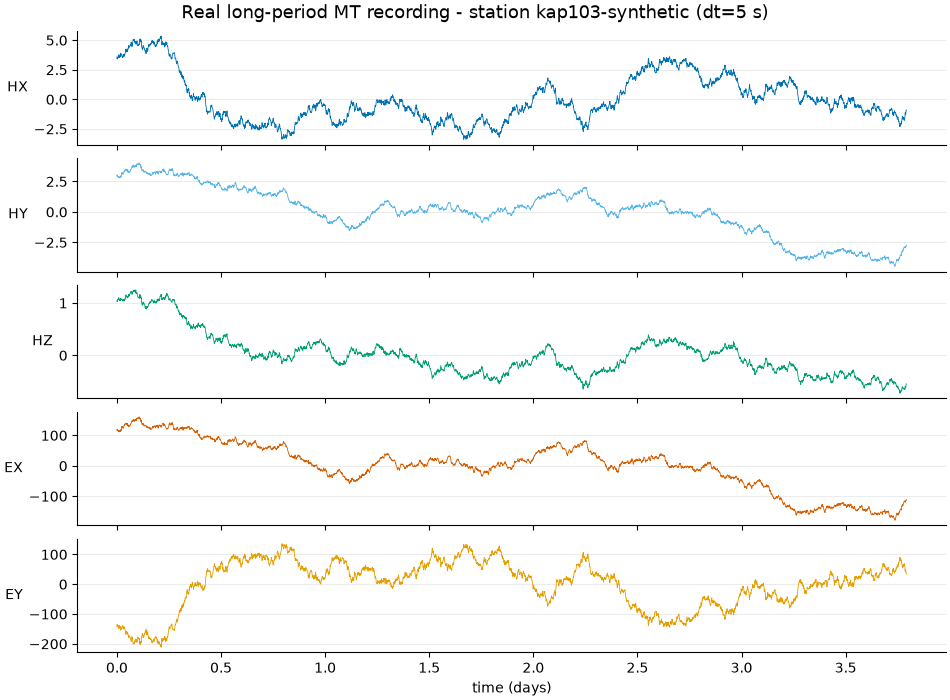
The raw channels reveal the recording’s real structure — slow MT variations plus true data gaps (drawn as breaks). Magnetic channels are cool, electric channels warm.

decim = max(1, record.n_samples // 4000)
t_days = np.arange(record.n_samples)[::decim] * record.dt / 86400.0

fig, axes = plt.subplots(
    len(channels), 1, figsize=(9.5, 7.0), sharex=True, constrained_layout=True
)
for ax, channel in zip(axes, channels):
    ax.plot(t_days, data[channel][::decim], lw=0.6, color=CH_COLORS[channel])
    ax.set_ylabel(channel.upper(), rotation=0, ha="right", va="center")
    style_axis(ax)
axes[-1].set_xlabel("time (days)")
fig.suptitle(
    f"Real long-period MT recording - station {record.station} (dt={record.dt:g} s)",
    fontsize=13,
)

Text(0.5, 0.9940471428571429, 'Real long-period MT recording - station kap103-synthetic (dt=5 s)')

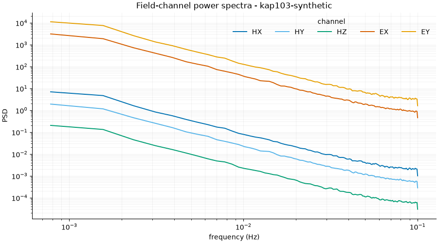
The power spectra show the field’s red MT spectrum. One shared log-log axis; identity is carried by a legend, never colour alone.

fig, ax = plt.subplots(figsize=(9.0, 5.0), constrained_layout=True)
for channel in channels:
    spec = compute_live_spectra(data[channel], sample_rate)
    freqs, psd = spec["frequency_hz"], spec["psd"]
    keep = freqs > 0
    ax.loglog(
        freqs[keep],
        psd[keep] + 1e-30,
        lw=1.4,
        color=CH_COLORS[channel],
        label=channel.upper(),
    )
ax.set(
    xlabel="frequency (Hz)",
    ylabel="PSD",
    title=f"Field-channel power spectra - {record.station}",
)
ax.legend(title="channel", ncol=5, frameon=False, loc="upper right")
style_axis(ax)
ax.grid(True, which="both", color="#000000", alpha=0.06, lw=0.6)

3. Fold the QC into the IoT edge layer

EdgeProcessor reduces the multi-channel block to a single QC result. A tight warn_finite_threshold turns the recording’s small real gaps into a WARNING rather than a silent pass — the field-QC state the generic ACCEPT/REJECT pair could not express.

block = np.column_stack([data[c] for c in channels])
processor = EdgeProcessor(
    EdgeProcessingConfig(finite_threshold=0.9, warn_finite_threshold=0.999)
)
result = processor.process(block, channel_names=channels)
print(
    f"edge decision: {result.decision.value}  "
    f"(coverage={result.metrics['finite_coverage']:.4f}, "
    f"warnings={result.metrics.get('warnings', 'none')})"
)

device = DeviceConfig(
    "kap103-recorder",
    station=record.station,
    channels=channels,
    sample_rate_hz=sample_rate,
)
session = FieldSession("KAP103-LP-MT", devices=[device], method="mt")
session.add_packet(result.to_packet(device, timestamp=1_720_000_000.0))
status = session.assess()
print(
    f"session assess: level={status.level.value}  "
    f"packets={status.n_packet}  "
    f"edge_acceptance_rate={status.edge_acceptance_rate:.2f}"
)

edge decision: accept  (coverage=1.0000, warnings=none)
session assess: level=ok  packets=1  edge_acceptance_rate=1.00

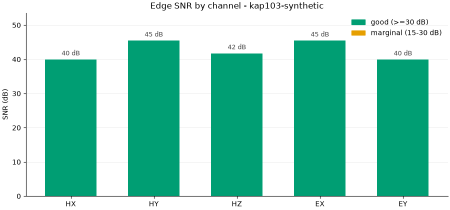
Coverage is shared across channels (whole-sample gaps), but SNR is not: the electric channels are markedly noisier than the magnetic ones — a real QC observation worth surfacing. Status colour is reserved and every bar is labelled, so state never rests on colour alone.

from matplotlib.patches import Patch  # noqa: E402

fig, ax = plt.subplots(figsize=(9.0, 4.2), constrained_layout=True)
labels = [r["channel"].upper() for r in rows]
snr = np.array([r["snr_db"] for r in rows])


def snr_color(value: float) -> str:
    if value >= 30.0:
        return STATUS["ok"]
    if value >= 15.0:
        return STATUS["warn"]
    return STATUS["bad"]


ax.bar(labels, snr, color=[snr_color(v) for v in snr], width=0.62)
for i, value in enumerate(snr):
    ax.text(
        i,
        value + 0.8,
        f"{value:.0f} dB",
        ha="center",
        va="bottom",
        fontsize=9,
        color="#444444",
    )
ax.set(
    ylabel="SNR (dB)",
    ylim=(0, snr.max() * 1.18),
    title=f"Edge SNR by channel - {record.station}",
)
ax.legend(
    handles=[
        Patch(color=STATUS["ok"], label="good (>=30 dB)"),
        Patch(color=STATUS["warn"], label="marginal (15-30 dB)"),
    ],
    frameon=False,
    loc="upper right",
)
style_axis(ax)

4. Reproducible provenance for the raw recording

Finally we hash the real .ts file and attach it to a provenance record, then export a manifest + audit bundle that can travel beside the raw data — the integrity trail reviewers expect.

provenance = ProvenanceRecord(
    station_id=record.station,
    sample_rate_hz=sample_rate,
    lat=record.lat,
    lon=record.lon,
    field_notes="Bundled SAMTEX/LiMS long-period MT test series.",
)
file_record = provenance.add_raw_file(str(ts_path)) if ts_is_real else None
manifest = build_acquisition_manifest(
    "KAP103-LP-MT", records=[provenance], method="mt"
)
bundle = export_reproducibility_bundle(
    manifest, str(Path(tempfile.gettempdir()) / "kap103_repro")
)
if file_record is not None:
    print(
        f"hashed {file_record['name']} "
        f"({file_record['bytes']:,} bytes) -> {file_record['digest'][:16]}..."
    )
else:
    print(
        "raw TS file not bundled — provenance hash skipped (synthetic sample)."
    )
print(f"manifest content hash: {manifest.as_dict()['content_hash'][:16]}...")
print(
    f"bundle: {Path(bundle['manifest']).name} "
    f"+ {len(bundle['audits'])} station audit(s)"
)

plt.show()

raw TS file not bundled — provenance hash skipped (synthetic sample).
manifest content hash: ecc658cda77228f2...
bundle: acquisition_manifest.json + 1 station audit(s)