Spectra EDI quality-control workflow

Most site workflows start from processed impedance EDI files: the file already contains Z and maybe a tipper. Spectra EDI files are more primitive and more informative. They store the cross-power spectral matrix from which impedance and tipper can be recovered.

This example uses the two bundled spectra files that are safe to ship in the repository:

data/MT/SPECTRA/spectra01.edi

Short-period / AMT-band spectra, from about 10400 Hz down to 1.72 Hz.

data/MT/SPECTRA/spectra02.edi

Broader and longer-period spectra, from about 320 Hz down to 0.00042 Hz.

The objective is to guide a user through a more sophisticated decision:

Can these spectra files support trustworthy transfer functions, and which frequency bands look most useful?

The workflow combines site-style thinking with spectra tools:

• inspect frequency/period coverage;

• compare PSD envelopes by channel family;

• score MT-relevant channel-pair coherence;

• build a pass/fail coherence mask;

• visualize the spectral matrix at representative frequencies;

• recover impedance and tipper from spectra;

• summarize the practical decision at the end.

1. Imports and data paths

The examples use public imports and keep the setup visible. The small path bootstrap lets this file run from a source checkout as well as inside the Sphinx gallery build.

import os
import sys
from pathlib import Path

import matplotlib.pyplot as plt
import numpy as np


def repo_root():
    root = os.environ.get("PYCSAMT_DOCS_REPO_ROOT")
    return Path(root) if root else Path(__file__).resolve().parents[3]


ROOT = repo_root()
if str(ROOT) not in sys.path:
    sys.path.insert(0, str(ROOT))

from pycsamt.emtools import (
    coherence_table,
    mask_low_coherence,
    plot_coherence_section,
    plot_spectra_matrix,
    plot_tipper_from_spectra,
    plot_z_from_spectra,
    psd_table,
)
from pycsamt.emtools.spectra import snr_table
from pycsamt.seg.spectra import Spectra

spectra_dir = ROOT / "data" / "MT" / "SPECTRA"
spectra_files = {
    "spectra01": spectra_dir / "spectra01.edi",
    "spectra02": spectra_dir / "spectra02.edi",
}
spectra = {
    name: Spectra.from_file(path) for name, path in spectra_files.items()
}

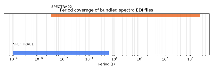
2. Coverage audit: frequency and period ranges

A spectra file is only useful for a workflow if its band overlaps the target period range. The first table is deliberately simple: station name, number of frequency blocks, frequency range, and equivalent period range.

coverage_rows = []
for label, sp in spectra.items():
    coverage_rows.append(
        {
            "label": label,
            "station": sp.name,
            "n_freq": sp.n_freq,
            "n_chan": sp.n_chan,
            "freq_min_hz": float(np.nanmin(sp.freq)),
            "freq_max_hz": float(np.nanmax(sp.freq)),
            "period_min_s": float(1.0 / np.nanmax(sp.freq)),
            "period_max_s": float(1.0 / np.nanmin(sp.freq)),
        }
    )

for row in coverage_rows:
    print(row)

{'label': 'spectra01', 'station': 'SPECTRA01', 'n_freq': 51, 'n_chan': 7, 'freq_min_hz': 1.72, 'freq_max_hz': 10400.0, 'period_min_s': 9.615384615384615e-05, 'period_max_s': 0.5813953488372093}
{'label': 'spectra02', 'station': 'SPECTRA02', 'n_freq': 73, 'n_chan': 7, 'freq_min_hz': 0.00042, 'freq_max_hz': 320.0, 'period_min_s': 0.003125, 'period_max_s': 2380.9523809523807}

The two files are complementary: spectra01 covers the high-frequency side, while spectra02 extends far into long periods. The following plot turns that into a visual band map.

fig, ax = plt.subplots(figsize=(8.5, 2.8))
for y, row in enumerate(coverage_rows):
    ax.hlines(
        y,
        row["period_min_s"],
        row["period_max_s"],
        lw=10,
        color=["#2563eb", "#ea580c"][y],
        alpha=0.75,
    )
    ax.text(row["period_min_s"], y + 0.18, row["station"], va="bottom")

ax.set_xscale("log")
ax.set_yticks([])
ax.set_xlabel("Period (s)")
ax.set_title("Period coverage of bundled spectra EDI files")
ax.grid(True, axis="x", which="both", alpha=0.25)
fig.tight_layout()

3. Choose MT-relevant channel pairs

The spectra files have seven channels: electric channels EX/EY, magnetic channels HX/HY/HZ, and duplicated horizontal magnetic channels that act like local reference channels.

For a compact MT decision metric, we focus on the usual off-diagonal pairs:

• EX with HY

• EY with HX

The helper below finds the first channel index for a channel type. That keeps the example robust to the station-specific channel IDs stored in the EDI header.

def first_channel_index(sp, channel_type):
    for index, key in enumerate(sp.id_to_chtype):
        if sp.id_to_chtype[key].upper() == channel_type.upper():
            return index
    raise KeyError(f"{sp.name} has no {channel_type!r} channel")


def mt_pairs(sp):
    ex = first_channel_index(sp, "EX")
    ey = first_channel_index(sp, "EY")
    hx = first_channel_index(sp, "HX")
    hy = first_channel_index(sp, "HY")
    return [(ex, hy), (ey, hx)]


for label, sp in spectra.items():
    print(label, sp.id_to_chtype)
    print("MT pairs:", mt_pairs(sp))

spectra01 {'31.003': 'HX', '32.003': 'HY', '33.003': 'HZ', '34.003': 'EX', '35.003': 'EY', '36.003': 'HX', '37.003': 'HY'}
MT pairs: [(3, 1), (4, 0)]
spectra02 {'021.002': 'HX', '022.002': 'HY', '023.002': 'HZ', '024.002': 'EX', '025.002': 'EY', '026.002': 'HX', '027.002': 'HY'}
MT pairs: [(3, 1), (4, 0)]

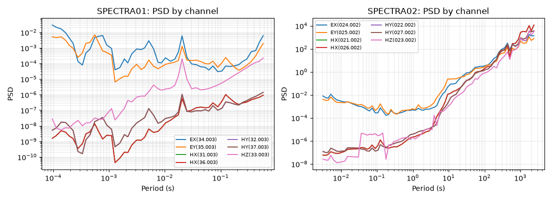
4. PSD envelopes by channel

Raw PSD amplitudes mix physical units, instrument response, and signal strength. The point of this plot is not to compare EX directly against HX in absolute units. The point is to see whether a channel family has sharp holes, unstable edges, or an obvious outlier station.

fig, axs = plt.subplots(1, 2, figsize=(11, 4), sharey=False)
for ax, (label, sp) in zip(axs, spectra.items()):
    psd = psd_table(sp)
    for channel, group in psd.groupby("channel"):
        ax.loglog(group["period"], group["psd"], lw=1.4, label=channel)
    ax.set_title(f"{sp.name}: PSD by channel")
    ax.set_xlabel("Period (s)")
    ax.set_ylabel("PSD")
    ax.grid(True, which="both", alpha=0.25)
    ax.legend(fontsize=7, ncol=2)
fig.tight_layout()

5. Coherence and SNR summary

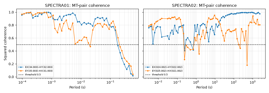
Squared coherence ranges from 0 to 1. Values near 1 mean two channels are strongly linearly related at that frequency; values near 0 mean the pair is not providing a stable transfer-function estimate.

snr_table converts the same coherence values into a coherence-based SNR estimate in dB, which is often easier to threshold in processing recipes.

coh_tables = {}
snr_tables = {}
for label, sp in spectra.items():
    pairs = mt_pairs(sp)
    coh = coherence_table(sp, pairs=pairs)
    snr = snr_table(sp, pairs=pairs)
    coh_tables[label] = coh
    snr_tables[label] = snr

    print(f"\n{sp.name} MT-pair coherence:")
    print(
        coh.groupby("pair")["coherence"].agg(["min", "median", "mean", "max"])
    )
    print(f"{sp.name} coherence-based SNR dB:")
    print(snr.groupby("pair")["snr_db"].agg(["median", "mean", "max"]))

SPECTRA01 MT-pair coherence:
                            min    median      mean       max
pair
EX(34.003)-HY(32.003)  0.018285  0.900658  0.797033  0.998137
EY(35.003)-HX(31.003)  0.041189  0.798813  0.728161  0.996734
SPECTRA01 coherence-based SNR dB:
                         median      mean        max
pair
EX(34.003)-HY(32.003)  9.574249  9.044718  27.288879
EY(35.003)-HX(31.003)  5.988465  6.879817  24.845567

SPECTRA02 MT-pair coherence:
                              min    median      mean       max
pair
EX(024.002)-HY(022.002)  0.404126  0.798644  0.811919  0.997414
EY(025.002)-HX(021.002)  0.182105  0.786114  0.738146  0.953366
SPECTRA02 coherence-based SNR dB:
                           median      mean        max
pair
EX(024.002)-HY(022.002)  5.983877  9.479798  25.862330
EY(025.002)-HX(021.002)  5.653042  5.256875  13.105529

A nicer visual is to plot coherence curves for both spectra files together, one panel per file. The dashed line marks a practical threshold used below.

threshold = 0.5
fig, axs = plt.subplots(1, 2, figsize=(11, 3.8), sharey=True)
for ax, (label, sp) in zip(axs, spectra.items()):
    coh = coh_tables[label]
    for pair, group in coh.groupby("pair"):
        ax.semilogx(
            group["period"],
            group["coherence"],
            marker=".",
            lw=1.2,
            label=pair,
        )
    ax.axhline(
        threshold, color="k", ls="--", lw=1, label=f"threshold {threshold:g}"
    )
    ax.set_title(f"{sp.name}: MT-pair coherence")
    ax.set_xlabel("Period (s)")
    ax.set_ylim(-0.02, 1.05)
    ax.grid(True, which="both", alpha=0.25)
    ax.legend(fontsize=7)
axs[0].set_ylabel("Squared coherence")
fig.tight_layout()

6. Frequency masks: which samples pass both MT pairs?

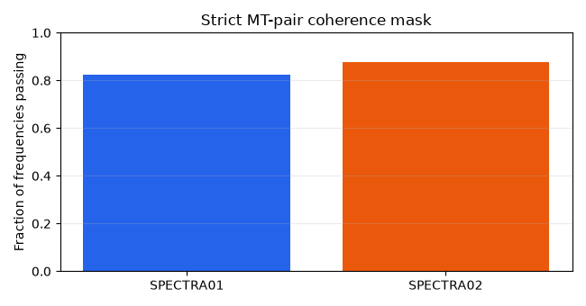
mask_low_coherence(..., require_all=True) keeps a frequency only when both MT-relevant pairs clear the threshold. This is stricter than asking whether either pair looks good.

mask_rows = []
for label, sp in spectra.items():
    mask = mask_low_coherence(
        sp,
        pairs=mt_pairs(sp),
        threshold=threshold,
        require_all=True,
    )
    periods = 1.0 / sp.freq
    passed_periods = periods[mask]
    mask_rows.append(
        {
            "label": label,
            "station": sp.name,
            "n_freq": int(sp.n_freq),
            "n_pass": int(mask.sum()),
            "pass_fraction": float(mask.mean()),
            "passed_period_min_s": float(np.nanmin(passed_periods))
            if mask.any()
            else np.nan,
            "passed_period_max_s": float(np.nanmax(passed_periods))
            if mask.any()
            else np.nan,
        }
    )

print("Strict coherence-mask summary:")
for row in mask_rows:
    print(row)

fig, ax = plt.subplots(figsize=(6.5, 3.4))
ax.bar(
    [row["station"] for row in mask_rows],
    [row["pass_fraction"] for row in mask_rows],
    color=["#2563eb", "#ea580c"],
)
ax.set_ylim(0, 1)
ax.set_ylabel("Fraction of frequencies passing")
ax.set_title("Strict MT-pair coherence mask")
ax.grid(axis="y", alpha=0.25)
fig.tight_layout()

Strict coherence-mask summary:
{'label': 'spectra01', 'station': 'SPECTRA01', 'n_freq': 51, 'n_pass': 42, 'pass_fraction': 0.8235294117647058, 'passed_period_min_s': 9.615384615384615e-05, 'passed_period_max_s': 0.14492753623188406}
{'label': 'spectra02', 'station': 'SPECTRA02', 'n_freq': 73, 'n_pass': 64, 'pass_fraction': 0.8767123287671232, 'passed_period_min_s': 0.003125, 'passed_period_max_s': 2380.9523809523807}

7. Cross-spectral matrix snapshots

The full spectral matrix is the raw object behind all later estimates. Plotting a representative matrix helps users see whether the energy is distributed sensibly across auto- and cross-channel terms.

plot_spectra_matrix(
    spectra["spectra01"],
    freq_idx=0,
    quantity="abs",
    title="spectra01: high-frequency spectral matrix",
)
plot_spectra_matrix(
    spectra["spectra02"],
    freq_idx=len(spectra["spectra02"].freq) // 2,
    quantity="abs",
    title="spectra02: mid-band spectral matrix",
)

• 
• 

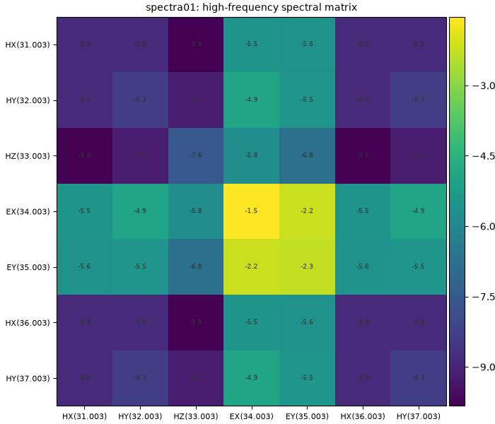
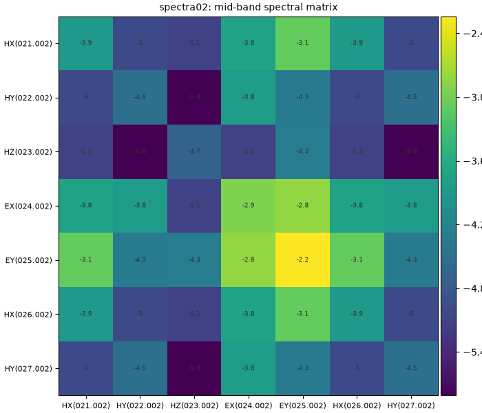
<Figure size 700x600 with 2 Axes>

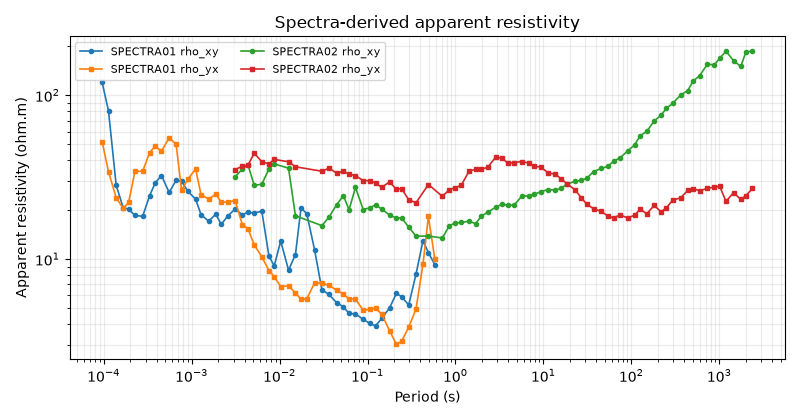
8. Recover impedance from spectra

plot_z_from_spectra calls Spectra.to_Z internally. We also compute the tensors directly so we can build a clean comparison plot of apparent resistivity for the two files.

for label, sp in spectra.items():
    plot_z_from_spectra(sp)

fig, ax = plt.subplots(figsize=(8, 4.2))
for label, sp in spectra.items():
    z, _tip = sp.to_Z(estimate_error=False)
    period = 1.0 / sp.freq
    rho = z.resistivity
    ax.loglog(
        period,
        rho[:, 0, 1],
        marker="o",
        ms=3,
        lw=1.2,
        label=f"{sp.name} rho_xy",
    )
    ax.loglog(
        period,
        rho[:, 1, 0],
        marker="s",
        ms=3,
        lw=1.2,
        label=f"{sp.name} rho_yx",
    )

ax.set_xlabel("Period (s)")
ax.set_ylabel("Apparent resistivity (ohm.m)")
ax.set_title("Spectra-derived apparent resistivity")
ax.grid(True, which="both", alpha=0.25)
ax.legend(fontsize=8, ncol=2)
fig.tight_layout()

• 
• 
• 

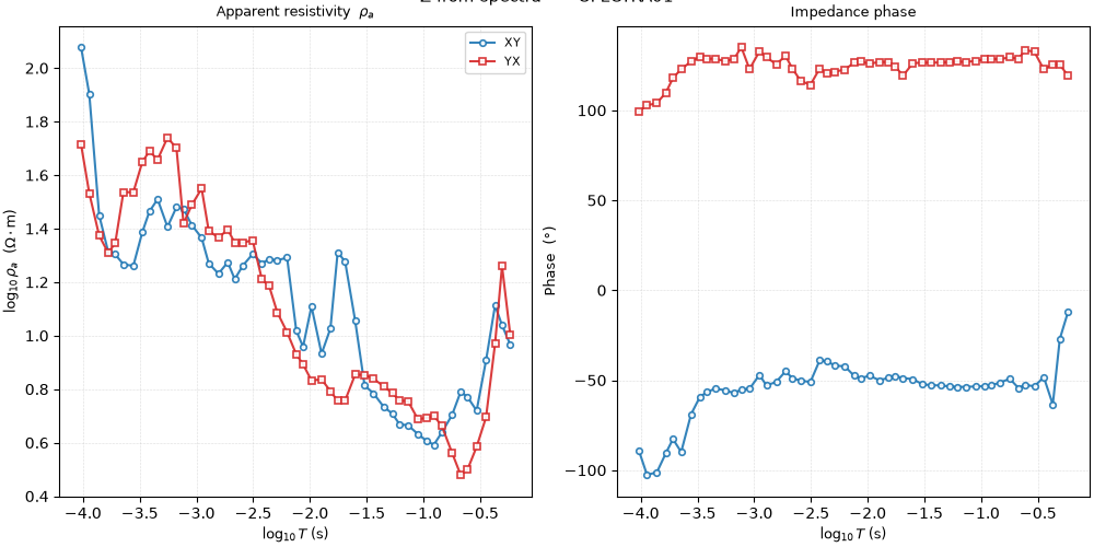
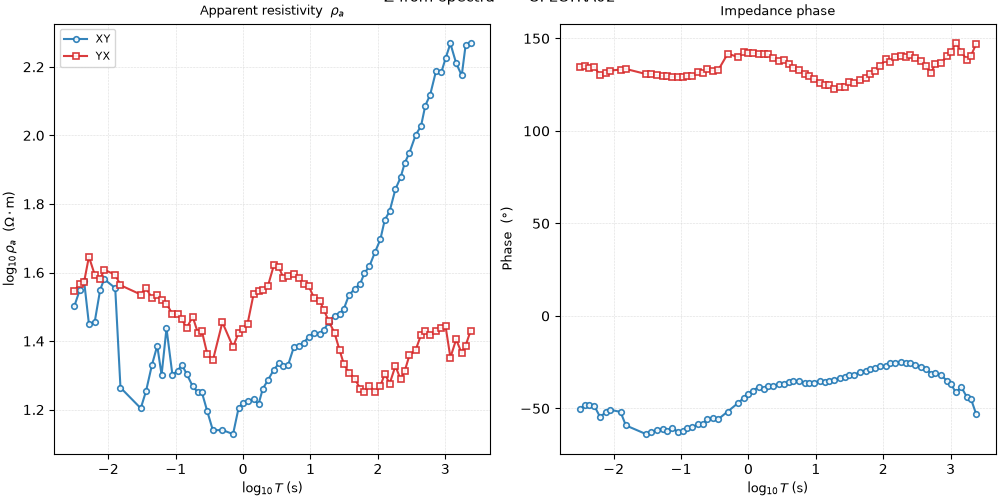
9. Recover tipper from spectra

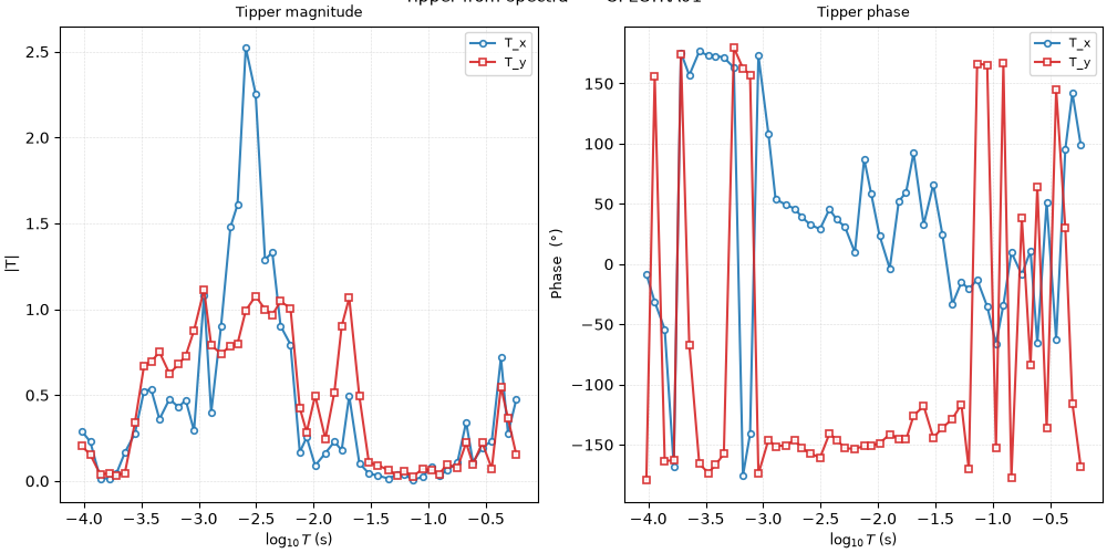
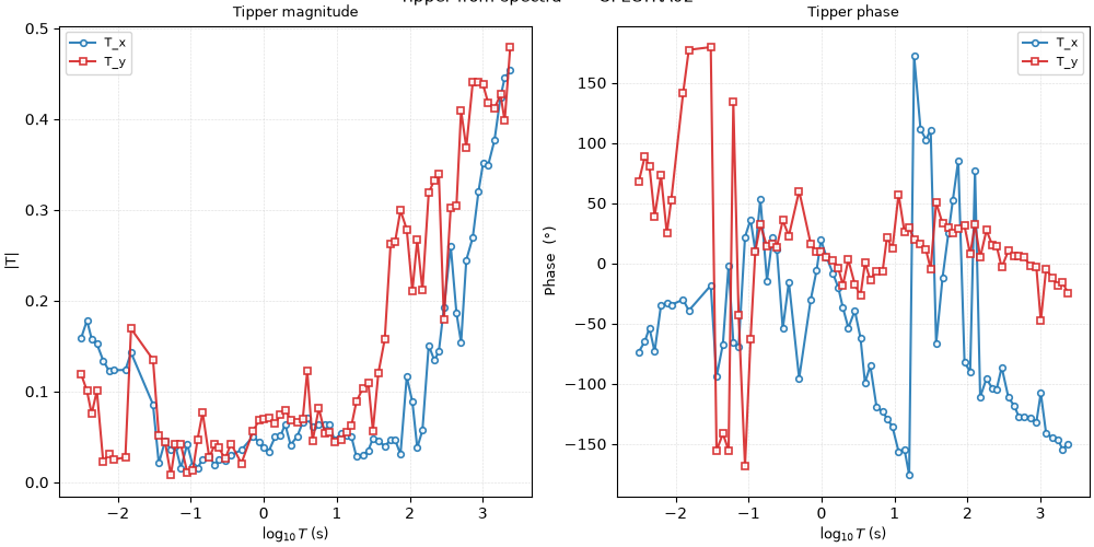
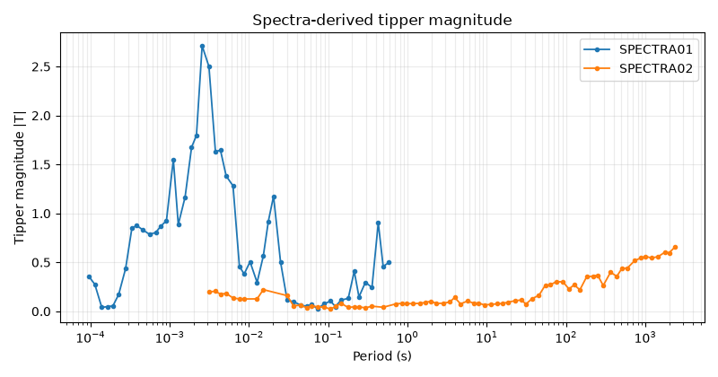
Because these spectra include HZ, pyCSAMT can also estimate the tipper. The standard helper gives a component plot; the custom summary below adds a compact magnitude comparison.

for label, sp in spectra.items():
    plot_tipper_from_spectra(sp)

fig, ax = plt.subplots(figsize=(8, 4.2))
for label, sp in spectra.items():
    _z, tip = sp.to_Z(estimate_error=False)
    period = 1.0 / sp.freq
    tip_arr = np.asarray(tip.tipper)
    if tip_arr.ndim == 3 and tip_arr.shape[1:] == (1, 2):
        tip_arr = tip_arr[:, 0, :]
    mag = np.sqrt(np.sum(np.abs(tip_arr) ** 2, axis=-1))
    ax.semilogx(period, mag, marker="o", ms=3, lw=1.3, label=sp.name)

ax.set_xlabel("Period (s)")
ax.set_ylabel("Tipper magnitude |T|")
ax.set_title("Spectra-derived tipper magnitude")
ax.grid(True, which="both", alpha=0.25)
ax.legend()
fig.tight_layout()

• 
• 
• 

10. Multi-station coherence section

The two files are not a full profile, but plotting them together still shows how pyCSAMT expects spectra collections to be compared across station-like inputs. This becomes more powerful when a directory contains many spectra EDI files.

ex_hy_pair = mt_pairs(spectra["spectra01"])[0]
plot_coherence_section(
    spectra,
    pair=ex_hy_pair,
    threshold=threshold,
    title="Bundled spectra files: EX-HY coherence section",
    figsize=(8, 4.5),
)

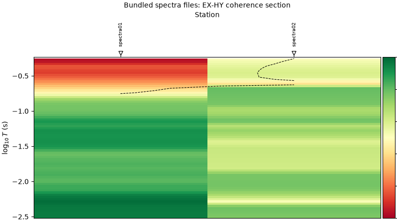
<Axes: title={'center': 'Bundled spectra files: EX-HY coherence section'}, xlabel='Station', ylabel='$\\log_{10}T$ (s)'>

11. Practical decision

This page is not just “make plots”; it is a decision workflow.

A user should leave with these conclusions:

• spectra01 is the high-frequency file and spectra02 reaches much longer periods.

• PSD plots reveal channel-family behavior, but coherence is the more direct transfer-function readiness check.

• The strict coherence mask is useful because it requires both MT pairs to pass at the same frequency.

• Impedance and tipper can be recovered from the spectra, but they should be interpreted together with the coherence diagnostics, not in isolation.

• For production, the same pattern can be wrapped around a directory of spectra EDI files before conversion to impedance EDI.