Detailed line case study with site-level diagnostics

This example is a more complete site/line study. Instead of only loading or filtering data, it uses pycsamt.site to build a small interpretation brief for one survey line.

The objective is:

choose one line, identify the most diagnostic station from the data, and make plots that explain why that station deserves follow-up.

The workflow is intentionally robust:

• load all WILLY lines, then isolate one line by station-name pattern;

• compute apparent resistivity at several target frequencies;

• derive simple screening attributes: off-diagonal anisotropy, phase slope, and quick strike proxy;

• build line-profile and station-frequency section plots;

• automatically select a station with strong contrast;

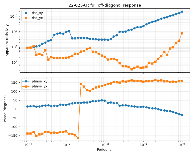
• inspect that station’s full resistivity/phase response.

These plots are not a replacement for full QC, static-shift correction, or inversion. They are a compact “what should I look at next?” study.

1. Imports and data setup

import os
import sys
from pathlib import Path

import matplotlib.pyplot as plt
import numpy as np


def repo_root():
    root = os.environ.get("PYCSAMT_DOCS_REPO_ROOT")
    return Path(root) if root else Path(__file__).resolve().parents[3]


ROOT = repo_root()
if str(ROOT) not in sys.path:
    sys.path.insert(0, str(ROOT))

from pycsamt.emtools import ensure_sites
from pycsamt.site import (
    SitesReport,
    by_names,
    keep_finite_z,
    phase_slope,
    res_at_freq,
    strike_estimate,
)

willy_dir = ROOT / "data" / "AMT" / "WILLY_DATA"
line_pattern = "22-*"
line_label = "L22"
target_frequencies = [10.0, 32.0, 100.0, 320.0, 1_000.0]
phase_band = (10.0, 1_000.0)

2. Load the survey and isolate one line

The WILLY station names encode the line prefix. by_names keeps the example readable and avoids hard-coding file paths to individual EDI files.

all_sites = ensure_sites(willy_dir, recursive=True, verbose=0)
all_sites = keep_finite_z(all_sites)
line_sites = by_names(all_sites, line_pattern)

if len(line_sites) == 0:
    raise RuntimeError(f"No stations matched {line_pattern!r}.")

line_report = SitesReport(line_sites).to_dataframe(api=False)
line_report["station_number"] = (
    line_report["station"].str.extract(r"-(\d+)", expand=False).astype(float)
)
line_report = line_report.sort_values("station_number")

print(f"{line_label} station count: {len(line_sites)}")
print(
    line_report[["station", "nfreq", "freq_min", "freq_max", "lat", "lon"]]
    .head()
    .to_string(index=False)
)

L22 station count: 25
station  nfreq  freq_min  freq_max       lat        lon
 22-1BF     53     1.008   10400.0 32.117900 119.126867
 22-2VF     53     1.008   10400.0 32.118433 119.126783
  22-3U     53     1.008   10400.0 32.119350 119.126750
  22-4U     53     1.008   10400.0 32.120283 119.126667
  22-5U     53     1.008   10400.0 32.121167 119.126717

3. Build a multi-frequency screening table

res_at_freq chooses the nearest available frequency for each station. We evaluate several frequencies to see whether a contrast persists across the band or only appears locally.

screen = line_report[
    ["station", "station_number", "lat", "lon", "nfreq"]
].copy()

for freq in target_frequencies:
    rho = res_at_freq(line_sites, freq, how="nearest", api=False)
    rho["rho_gmean"] = np.sqrt(rho["res_xy"] * rho["res_yx"])
    rho["rho_anisotropy"] = np.abs(np.log10(rho["res_xy"] / rho["res_yx"]))
    suffix = f"{int(freq):04d}hz"
    screen = screen.merge(
        rho[["station", "rho_gmean", "rho_anisotropy", "f_used"]],
        on="station",
        how="left",
    ).rename(
        columns={
            "rho_gmean": f"rho_{suffix}",
            "rho_anisotropy": f"anis_{suffix}",
            "f_used": f"f_used_{suffix}",
        }
    )

slopes = phase_slope(line_sites, phase_band, api=False)
strike = strike_estimate(line_sites, method="phase_diff", api=False)
screen = screen.merge(slopes, on="station", how="left")
screen = screen.merge(
    strike[["station", "theta_deg"]], on="station", how="left"
)
screen["phase_slope_abs"] = (
    screen[["slope_xy", "slope_yx"]].abs().mean(axis=1)
)

print("Screening table preview:")
print(
    screen[
        [
            "station",
            "rho_0100hz",
            "anis_0100hz",
            "phase_slope_abs",
            "theta_deg",
        ]
    ]
    .head(10)
    .to_string(index=False)
)

Screening table preview:
station   rho_0100hz  anis_0100hz  phase_slope_abs  theta_deg
 22-1BF 9.749634e+07     0.198859         1.727270        0.0
 22-2VF 4.755009e+07     0.359369         2.357386        0.0
  22-3U 2.707954e+08     1.078268         5.124809       90.0
  22-4U 3.249677e+08     0.887110         4.441426       90.0
  22-5U 2.020950e+08     0.068091         4.058975       90.0
  22-6U 8.303609e+07     0.427724         5.406299       90.0
  22-7U 9.850470e+07     0.067150         7.617378       90.0
  22-8U 1.819972e+08     0.137911         4.824884       90.0
  22-9A 1.747951e+08     0.038435        11.675905       90.0
 22-10U 2.375564e+08     0.022937         8.164376       90.0

4. Geometry and target-frequency map/profile

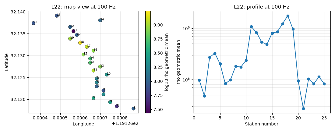
First check whether the line geometry is usable. The left plot uses header coordinates; the right plot uses station number as an along-line coordinate.

fig, axs = plt.subplots(1, 2, figsize=(11, 4.3))

sc = axs[0].scatter(
    screen["lon"],
    screen["lat"],
    c=np.log10(screen["rho_0100hz"]),
    s=70,
    cmap="viridis",
    edgecolor="black",
    linewidth=0.4,
)
for _, row in screen.iterrows():
    axs[0].text(
        row["lon"], row["lat"], str(int(row["station_number"])), fontsize=7
    )
axs[0].set_title(f"{line_label}: map view at 100 Hz")
axs[0].set_xlabel("Longitude")
axs[0].set_ylabel("Latitude")
axs[0].grid(alpha=0.25)
fig.colorbar(sc, ax=axs[0], label="log10 rho geometric mean")

axs[1].semilogy(
    screen["station_number"], screen["rho_0100hz"], marker="o", lw=1.6
)
axs[1].set_title(f"{line_label}: profile at 100 Hz")
axs[1].set_xlabel("Station number")
axs[1].set_ylabel("rho geometric mean")
axs[1].grid(True, which="both", alpha=0.25)

fig.tight_layout()

5. Multi-frequency line profiles

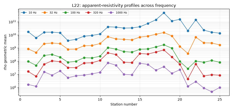
If a station is anomalous at every frequency, it may indicate a persistent structure. If it appears only at one end of the band, it may be a frequency-local effect or a data-quality issue.

fig, ax = plt.subplots(figsize=(9.5, 4.5))
for freq in target_frequencies:
    suffix = f"{int(freq):04d}hz"
    ax.semilogy(
        screen["station_number"],
        screen[f"rho_{suffix}"],
        marker="o",
        lw=1.3,
        label=f"{freq:g} Hz",
    )

ax.set_title(f"{line_label}: apparent-resistivity profiles across frequency")
ax.set_xlabel("Station number")
ax.set_ylabel("rho geometric mean")
ax.grid(True, which="both", alpha=0.25)
ax.legend(ncol=5, fontsize=8)
fig.tight_layout()

6. Station-frequency resistivity section

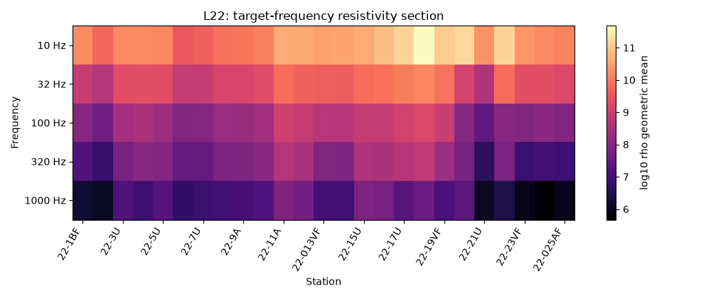
A heatmap gives a compact view of all selected frequencies and stations.

rho_matrix = np.vstack(
    [
        screen[f"rho_{int(freq):04d}hz"].to_numpy(dtype=float)
        for freq in target_frequencies
    ]
)

fig, ax = plt.subplots(figsize=(10, 4.2))
im = ax.imshow(np.log10(rho_matrix), aspect="auto", cmap="magma")
ax.set_yticks(np.arange(len(target_frequencies)))
ax.set_yticklabels([f"{f:g} Hz" for f in target_frequencies])
ax.set_xticks(np.arange(len(screen))[::2])
ax.set_xticklabels(screen["station"].iloc[::2], rotation=60, ha="right")
ax.set_title(f"{line_label}: target-frequency resistivity section")
ax.set_xlabel("Station")
ax.set_ylabel("Frequency")
fig.colorbar(im, ax=ax, label="log10 rho geometric mean")
fig.tight_layout()

7. Pick a diagnostic station automatically

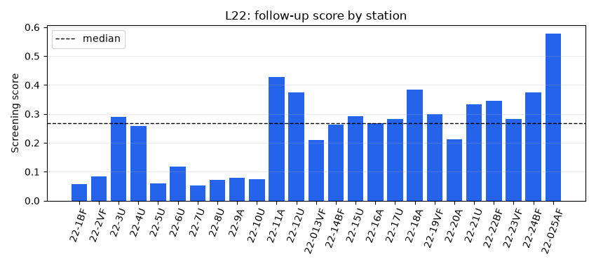
The score below combines high 100 Hz resistivity, high off-diagonal anisotropy, and high phase-slope magnitude. It is deliberately simple and transparent, not a hidden machine-learning decision.

score_parts = []
for column in ["rho_0100hz", "anis_0100hz", "phase_slope_abs"]:
    values = screen[column].to_numpy(dtype=float)
    lo = np.nanmin(values)
    hi = np.nanmax(values)
    score_parts.append((values - lo) / (hi - lo + 1e-12))

screen["followup_score"] = np.mean(score_parts, axis=0)
selected = screen.sort_values("followup_score", ascending=False).iloc[0]
selected_station = selected["station"]

print(f"Selected diagnostic station: {selected_station}")
print(
    selected[
        [
            "station",
            "rho_0100hz",
            "anis_0100hz",
            "phase_slope_abs",
            "theta_deg",
            "followup_score",
        ]
    ].to_string()
)

Selected diagnostic station: 22-025AF
station                   22-025AF
rho_0100hz         82660513.330379
anis_0100hz               1.126366
phase_slope_abs          79.830635
theta_deg                      0.0
followup_score            0.577162

Visualize why that station was selected.

fig, ax = plt.subplots(figsize=(8.5, 3.8))
ax.bar(screen["station"], screen["followup_score"], color="#2563eb")
ax.axhline(
    screen["followup_score"].median(),
    color="black",
    ls="--",
    lw=1,
    label="median",
)
ax.set_title(f"{line_label}: follow-up score by station")
ax.set_ylabel("Screening score")
ax.tick_params(axis="x", rotation=70)
ax.grid(axis="y", alpha=0.25)
ax.legend()
fig.tight_layout()

8. Full response curves for the selected station

Now inspect the selected station across its native frequency grid. We access the EDI object’s impedance tensor directly because this is a focused station-level diagnostic rather than a summary table.

def find_station(sites, name):
    for edi in sites.as_list():
        station = getattr(edi, "station", "") or getattr(
            getattr(edi, "Head", None), "dataid", ""
        )
        if station == name:
            return edi
    raise KeyError(name)


def z_and_freq(edi):
    z_obj = getattr(edi, "Z", None)
    freq = np.asarray(
        getattr(z_obj, "freq", getattr(z_obj, "_freq", [])), dtype=float
    )
    z = np.asarray(
        getattr(z_obj, "z", getattr(z_obj, "_z", [])), dtype=complex
    )
    order = np.argsort(freq)
    return freq[order], z[order]


edi = find_station(line_sites, selected_station)
freq, z = z_and_freq(edi)
period = 1.0 / freq

mu0 = 4.0 * np.pi * 1e-7
rho_xy = np.abs(z[:, 0, 1]) ** 2 / (mu0 * 2.0 * np.pi * freq)
rho_yx = np.abs(z[:, 1, 0]) ** 2 / (mu0 * 2.0 * np.pi * freq)
phi_xy = np.degrees(np.angle(z[:, 0, 1]))
phi_yx = np.degrees(np.angle(z[:, 1, 0]))

fig, axs = plt.subplots(2, 1, figsize=(8.2, 6.6), sharex=True)
axs[0].loglog(period, rho_xy, marker="o", lw=1.4, label="rho_xy")
axs[0].loglog(period, rho_yx, marker="s", lw=1.4, label="rho_yx")
axs[0].set_ylabel("Apparent resistivity")
axs[0].set_title(f"{selected_station}: full off-diagonal response")
axs[0].grid(True, which="both", alpha=0.25)
axs[0].legend()

axs[1].semilogx(period, phi_xy, marker="o", lw=1.4, label="phase_xy")
axs[1].semilogx(period, phi_yx, marker="s", lw=1.4, label="phase_yx")
axs[1].set_xlabel("Period (s)")
axs[1].set_ylabel("Phase (degrees)")
axs[1].grid(True, which="both", alpha=0.25)
axs[1].legend()
fig.tight_layout()

9. How to read this case study

The selected station is not declared “good” or “bad” by this page. It is declared interesting. The combination of target-frequency contrast, off-diagonal disagreement, and phase behavior makes it a good candidate for follow-up with:

• explicit QC scoring;

• static-shift checks;

• dimensionality and strike analysis;

• comparison with neighbouring stations;

• inversion only after the earlier checks are understood.

That is where site is most useful: it gives a lightweight, reproducible bridge between raw station collections and heavier interpretation tools.