Extracting topography from survey stations

Topography enters pyCSAMT through station metadata: latitude, longitude, and elevation stored in EDI headers or attached to site collections. Before using terrain in a section plot or inversion export, first check whether the station line has meaningful elevation and profile geometry.

This example answers:

Does this survey line carry usable elevation, and what does its terrain profile look like?

We use the bundled WILLY L18PLT line because its EDI headers contain real station elevations.

1. Imports and data loading

import os
import sys
from pathlib import Path

import matplotlib.pyplot as plt
import numpy as np


def repo_root():
    root = os.environ.get("PYCSAMT_DOCS_REPO_ROOT")
    return Path(root) if root else Path(__file__).resolve().parents[3]


ROOT = repo_root()
if str(ROOT) not in sys.path:
    sys.path.insert(0, str(ROOT))

from pycsamt.emtools import ensure_sites
from pycsamt.topo import (
    extract_chainage,
    extract_elevation,
    extract_station_names,
    has_elevation,
    interp_elev,
)

edi_dir = ROOT / "data" / "AMT" / "WILLY_DATA" / "L18PLT"
sites = ensure_sites(edi_dir, recursive=False, verbose=0)

2. Extract station names, chainage, and elevation

extract_chainage computes cumulative along-profile distance in kilometres from station coordinates. extract_elevation returns elevations in metres above sea level.

names = extract_station_names(sites)
chain_km = extract_chainage(sites)
elev_m = extract_elevation(sites)

print(f"Stations: {len(names)}")
print(f"Has non-zero elevation: {has_elevation(sites)}")
print(f"Profile length: {chain_km[-1]:.3f} km")
print(f"Elevation range: {elev_m.min():.1f} to {elev_m.max():.1f} m")

Stations: 28
Has non-zero elevation: True
Profile length: 19.662 km
Elevation range: 37.0 to 144.0 m

Build a small table for the first stations.

for row in zip(names[:8], chain_km[:8], elev_m[:8]):
    print(f"{row[0]:>8s}  chain={row[1]:6.3f} km  elev={row[2]:6.1f} m")

18-015U  chain= 0.000 km  elev= 103.0 m
18-008U  chain= 0.701 km  elev= 106.0 m
18-003A  chain= 1.204 km  elev=  81.0 m
18-016A  chain= 2.507 km  elev=  71.0 m
18-025A  chain= 3.410 km  elev=  81.0 m
18-023A  chain= 3.615 km  elev=  69.0 m
18-018A  chain= 4.115 km  elev=  72.0 m
18-010U  chain= 4.914 km  elev= 129.0 m

3. Station spacing and terrain slope

A topography overlay is most useful when the line geometry is trustworthy. Check both station spacing and local terrain slope before drawing it on a section.

spacing_m = np.diff(chain_km) * 1000.0
relief_m = np.diff(elev_m)
slope_deg = np.degrees(np.arctan2(relief_m, spacing_m))

print(f"Median station spacing: {np.median(spacing_m):.1f} m")
print(f"Maximum station spacing: {np.max(spacing_m):.1f} m")
print(
    f"Maximum absolute terrain slope: {np.max(np.abs(slope_deg)):.1f} degrees"
)

Median station spacing: 701.2 m
Maximum station spacing: 1898.2 m
Maximum absolute terrain slope: 7.6 degrees

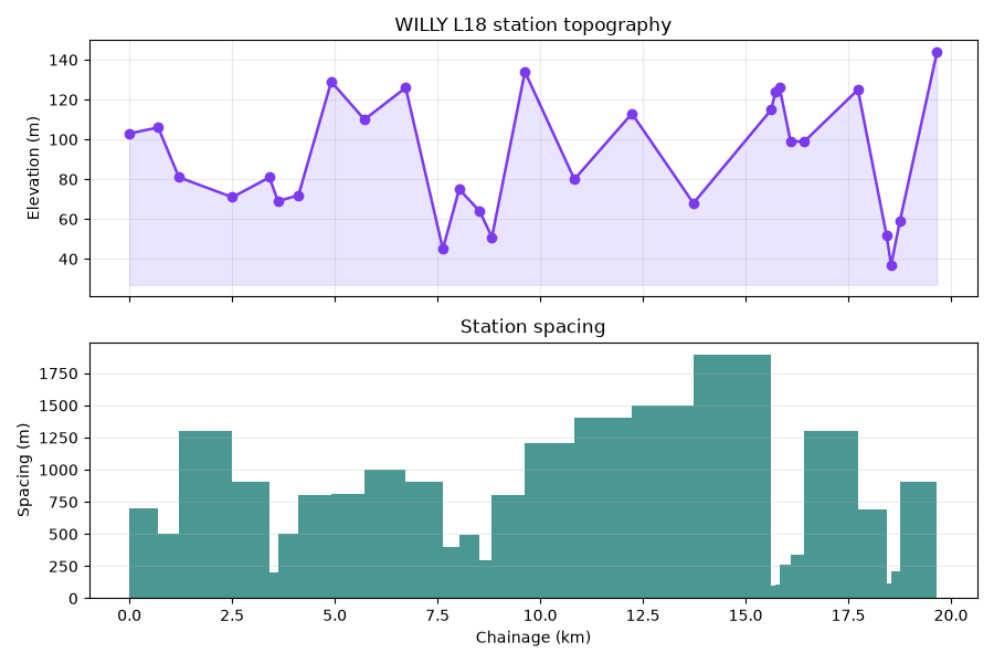
4. Plot the elevation profile

fig, axs = plt.subplots(2, 1, figsize=(9, 6), sharex=True)

axs[0].plot(chain_km, elev_m, marker="o", lw=1.8, color="#7c3aed")
axs[0].fill_between(
    chain_km, elev_m, elev_m.min() - 10, color="#c4b5fd", alpha=0.35
)
axs[0].set_ylabel("Elevation (m)")
axs[0].set_title("WILLY L18 station topography")
axs[0].grid(alpha=0.25)

axs[1].bar(
    chain_km[:-1],
    spacing_m,
    width=np.diff(chain_km),
    align="edge",
    color="#0f766e",
    alpha=0.75,
)
axs[1].set_xlabel("Chainage (km)")
axs[1].set_ylabel("Spacing (m)")
axs[1].set_title("Station spacing")
axs[1].grid(axis="y", alpha=0.25)

fig.tight_layout()

5. Interpolate elevation for section grids

Section meshes usually have many more x positions than station locations. interp_elev interpolates station elevation to arbitrary profile positions and clamps extrapolated edges to the boundary stations.

x_query = np.linspace(chain_km.min(), chain_km.max(), 200)
elev_query_km = interp_elev(chain_km, elev_m / 1000.0, x_query)

fig, ax = plt.subplots(figsize=(9, 3.4))
ax.plot(
    x_query,
    elev_query_km * 1000.0,
    color="#111827",
    lw=2,
    label="interpolated",
)
ax.scatter(
    chain_km,
    elev_m,
    s=45,
    color="#f97316",
    edgecolor="black",
    label="stations",
)
ax.set_xlabel("Chainage (km)")
ax.set_ylabel("Elevation (m)")
ax.set_title("Interpolated topography for downstream section meshes")
ax.grid(alpha=0.25)
ax.legend()
fig.tight_layout()

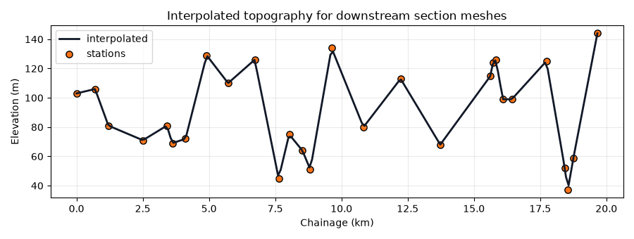
This first topo step is intentionally simple: verify the station elevation contract before drawing or draping a section. The next examples use the same arrays to build terrain-aware 2-D views.