Topo-aware pseudosections with emtools

The earlier topo examples used the low-level functions directly: extract_elevation, drape_section, and draw_topo_strip. In normal analysis, topography often enters through a higher-level plotting function.

This example shows that integration point:

use :mod:`pycsamt.topo` to audit station elevation, then let :func:`pycsamt.emtools.pseudosection` add the topography strip.

The workflow is robust because it does not simply switch topo=True and hope for the best. It first checks whether the line has usable elevation, computes profile geometry, identifies steep segments, and only then draws topography-aware pseudosections.

1. Imports and data

import os
import sys
from pathlib import Path

import matplotlib.pyplot as plt
import numpy as np


def repo_root():
    root = os.environ.get("PYCSAMT_DOCS_REPO_ROOT")
    return Path(root) if root else Path(__file__).resolve().parents[3]


ROOT = repo_root()
if str(ROOT) not in sys.path:
    sys.path.insert(0, str(ROOT))

from pycsamt.emtools import ensure_sites, pseudosection
from pycsamt.site import SitesReport
from pycsamt.topo import (
    PYCSAMT_TOPO,
    extract_chainage,
    extract_elevation,
    extract_station_names,
    has_elevation,
)

line_dir = ROOT / "data" / "AMT" / "WILLY_DATA" / "L18PLT"
sites = ensure_sites(line_dir, recursive=False, verbose=0)

2. Pre-flight topography audit

Higher-level plotting functions should not be responsible for deciding whether a terrain overlay is meaningful. Do the simple checks first.

names = extract_station_names(sites)
chain_km = extract_chainage(sites)
elev_m = extract_elevation(sites)
summary = SitesReport(sites).to_dataframe(api=False)

print(f"Stations: {len(names)}")
print(f"Has usable elevation: {has_elevation(sites)}")
print(
    f"Frequency rows per station: {summary['nfreq'].min()}-{summary['nfreq'].max()}"
)
print(f"Profile length: {chain_km[-1]:.3f} km")
print(f"Elevation range: {elev_m.min():.1f}-{elev_m.max():.1f} m")

if len(names) < 2:
    raise RuntimeError("Need at least two stations for a topo-aware profile.")
if not has_elevation(sites):
    raise RuntimeError("This example expects non-zero station elevations.")

Stations: 28
Has usable elevation: True
Frequency rows per station: 53-53
Profile length: 19.662 km
Elevation range: 37.0-144.0 m

3. Find geometry segments to inspect

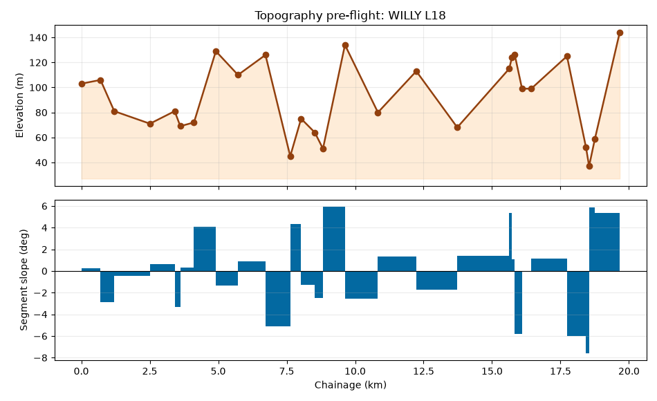
A topography strip is most useful when it highlights real geometry. The table below identifies the steepest station-to-station elevation changes.

spacing_m = np.diff(chain_km) * 1000.0
relief_m = np.diff(elev_m)
slope_deg = np.degrees(np.arctan2(relief_m, spacing_m))

segments = []
for i, slope in enumerate(slope_deg):
    segments.append(
        {
            "from": names[i],
            "to": names[i + 1],
            "spacing_m": spacing_m[i],
            "relief_m": relief_m[i],
            "slope_deg": slope,
        }
    )

segments = sorted(
    segments, key=lambda row: abs(row["slope_deg"]), reverse=True
)
print("Steepest station-to-station segments:")
for row in segments[:5]:
    print(row)

Steepest station-to-station segments:
{'from': '18-021U', 'to': '18-020A', 'spacing_m': np.float64(112.58073494141385), 'relief_m': np.float64(-15.0), 'slope_deg': np.float64(-7.589260530727813)}
{'from': '18-014A', 'to': '18-021U', 'spacing_m': np.float64(695.6070566596786), 'relief_m': np.float64(-73.0), 'slope_deg': np.float64(-5.990936712679023)}
{'from': '18-019U', 'to': '18-011A', 'spacing_m': np.float64(802.9244541658329), 'relief_m': np.float64(83.0), 'slope_deg': np.float64(5.901823657734221)}
{'from': '18-020A', 'to': '18-022V', 'spacing_m': np.float64(213.3260283251417), 'relief_m': np.float64(22.0), 'slope_deg': np.float64(5.888014486699096)}
{'from': '18-007U', 'to': '18-004A', 'spacing_m': np.float64(264.5546386262492), 'relief_m': np.float64(-27.0), 'slope_deg': np.float64(-5.8273341581590525)}

A compact geometry panel makes the later pseudosection easier to read.

fig, axs = plt.subplots(2, 1, figsize=(9.5, 5.8), sharex=True)

axs[0].plot(chain_km, elev_m, marker="o", color="#92400e", lw=1.8)
axs[0].fill_between(
    chain_km, elev_m, elev_m.min() - 10, color="#fed7aa", alpha=0.45
)
axs[0].set_ylabel("Elevation (m)")
axs[0].set_title("Topography pre-flight: WILLY L18")
axs[0].grid(alpha=0.25)

axs[1].bar(
    chain_km[:-1],
    slope_deg,
    width=np.diff(chain_km),
    align="edge",
    color="#0369a1",
)
axs[1].axhline(0, color="black", lw=0.8)
axs[1].set_xlabel("Chainage (km)")
axs[1].set_ylabel("Segment slope (deg)")
axs[1].grid(axis="y", alpha=0.25)

fig.tight_layout()

4. Compare pseudosections without and with topo

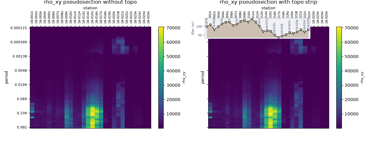
Frequency/period pseudosections do not have an elevation axis, so the correct topographic representation is a strip above the image, not a draped main panel. pseudosection(..., topo=True) delegates that strip to pycsamt.topo.

fig, axs = plt.subplots(1, 2, figsize=(12, 4.8), sharey=True)

pseudosection(
    sites,
    quantity="rho_xy",
    axis_x="station",
    axis_y="period",
    period_range=(1e-4, 1.0),
    ax=axs[0],
    topo=False,
    dark=False,
)
axs[0].set_title("rho_xy pseudosection without topo")

pseudosection(
    sites,
    quantity="rho_xy",
    axis_x="station",
    axis_y="period",
    period_range=(1e-4, 1.0),
    ax=axs[1],
    topo=True,
    dark=False,
)
axs[1].set_title("rho_xy pseudosection with topo strip")

fig.subplots_adjust(top=0.82, bottom=0.14, left=0.08, right=0.96, wspace=0.18)

5. Use global topo configuration intentionally

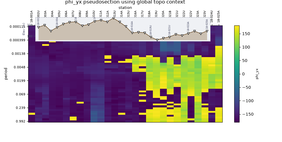
Some plotting workflows use the global singleton instead of passing topo=True each time. The context manager keeps that setting local to the current block, so one example does not silently affect the next one.

print("Global topo enabled before context:", PYCSAMT_TOPO.enabled)

with PYCSAMT_TOPO.context(
    enabled=True, strip_height_ratio=0.22, exaggeration=1.8
):
    fig, ax = plt.subplots(figsize=(9.5, 4.8))
    pseudosection(
        sites,
        quantity="phi_yx",
        axis_x="station",
        axis_y="period",
        period_range=(1e-4, 1.0),
        ax=ax,
        topo=None,
        dark=False,
    )
    ax.set_title("phi_yx pseudosection using global topo context")
    fig.subplots_adjust(top=0.82, bottom=0.14, left=0.10, right=0.96)

print("Global topo enabled after context:", PYCSAMT_TOPO.enabled)

Global topo enabled before context: False
Global topo enabled after context: False

6. When to use each topo display

Use this rule of thumb:

• Use pseudosection(..., topo=True) or draw_topo_strip when the vertical axis is period, frequency, station index, or another non-elevation coordinate.

• Use drape_section and draw_topo_section when the vertical axis is actual depth/elevation.

The strip is not a model surface. It is a context panel that tells the reader how station elevation changes along the same profile shown in the pseudosection.