Topo case study: from station relief to interpretation panels

Topography is not only a nice decoration above a plot. On a rough line it changes how we communicate the position of shallow conductors, resistive basement, and station coverage. This case study uses one WILLY profile and builds a small interpretation workflow around the terrain information stored in the EDI files.

The objective is to answer three practical questions before publishing a section:

• Does the line have reliable elevation values?

• Where is the topography strong enough to affect interpretation?

• How does a flat-depth section differ from a terrain-following section?

The numerical model below is synthetic. It is deliberately built from the station geometry so that the example remains lightweight and reproducible for the documentation gallery. In a real project the same plotting pattern can be applied to an inversion result, DOI grid, sensitivity section, or any 2-D image whose x-axis is chainage and whose vertical axis is depth.

1. Imports and line loading

Keep all imports at the top. Gallery examples are easier to copy when the dependencies are visible before the workflow starts.

import os
import sys
from pathlib import Path

import matplotlib.pyplot as plt
import numpy as np


def repo_root():
    root = os.environ.get("PYCSAMT_DOCS_REPO_ROOT")
    return Path(root) if root else Path(__file__).resolve().parents[3]


ROOT = repo_root()
if str(ROOT) not in sys.path:
    sys.path.insert(0, str(ROOT))

from pycsamt.emtools import ensure_sites
from pycsamt.site import SitesReport
from pycsamt.topo import (
    TopoConfig,
    drape_section,
    draw_topo_section,
    extract_chainage,
    extract_elevation,
    extract_station_names,
    has_elevation,
    interp_elev,
)

line_dir = ROOT / "data" / "AMT" / "WILLY_DATA" / "L18PLT"
sites = ensure_sites(line_dir, recursive=False, verbose=0)

2. Audit the topographic profile

Do this audit before drawing a terrain-aware figure. It gives the reader confidence that the terrain panel is based on station metadata, not on a hand-drawn curve.

names = extract_station_names(sites)
chain_km = extract_chainage(sites)
elev_m = extract_elevation(sites)
report = SitesReport(sites).to_dataframe(api=False)

if len(names) < 3:
    raise RuntimeError("This case study needs at least three stations.")
if not has_elevation(sites):
    raise RuntimeError(
        "The selected profile does not contain usable elevation."
    )

spacing_m = np.diff(chain_km) * 1000.0
relief_m = np.diff(elev_m)
slope_deg = np.degrees(np.arctan2(relief_m, spacing_m))

print("Topo case-study line:", line_dir.name)
print(f"Stations: {len(names)}")
print(f"Profile length: {chain_km[-1]:.3f} km")
print(f"Elevation range: {elev_m.min():.1f}-{elev_m.max():.1f} m")
print(f"Relief: {np.ptp(elev_m):.1f} m")
print(f"Median station spacing: {np.median(spacing_m):.1f} m")
print(
    f"Frequency rows per station: {report['nfreq'].min()}-{report['nfreq'].max()}"
)

steep = np.argsort(np.abs(slope_deg))[::-1][:6]
print("Steepest local segments:")
for i in steep:
    print(
        f"  {names[i]} -> {names[i + 1]}: "
        f"spacing={spacing_m[i]:.1f} m, relief={relief_m[i]:+.1f} m, "
        f"slope={slope_deg[i]:+.1f} deg"
    )

Topo case-study line: L18PLT
Stations: 28
Profile length: 19.662 km
Elevation range: 37.0-144.0 m
Relief: 107.0 m
Median station spacing: 701.2 m
Frequency rows per station: 53-53
Steepest local segments:
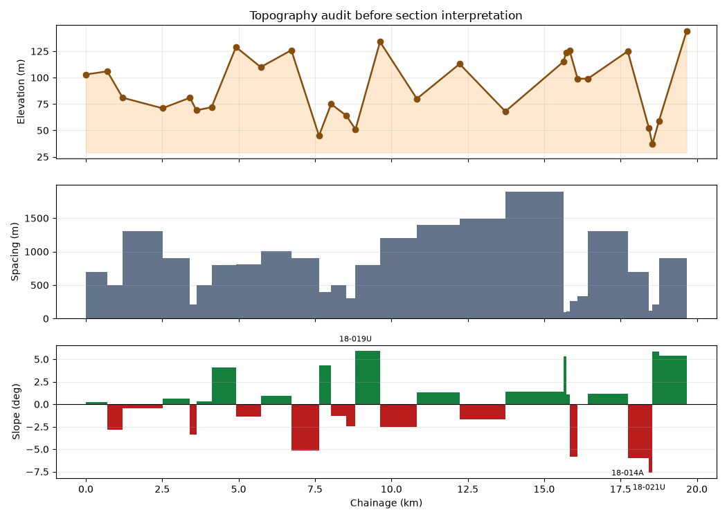
  18-021U -> 18-020A: spacing=112.6 m, relief=-15.0 m, slope=-7.6 deg
  18-014A -> 18-021U: spacing=695.6 m, relief=-73.0 m, slope=-6.0 deg
  18-019U -> 18-011A: spacing=802.9 m, relief=+83.0 m, slope=+5.9 deg
  18-020A -> 18-022V: spacing=213.3 m, relief=+22.0 m, slope=+5.9 deg
  18-007U -> 18-004A: spacing=264.6 m, relief=-27.0 m, slope=-5.8 deg
  18-022V -> 18-013U: spacing=904.7 m, relief=+85.0 m, slope=+5.4 deg

3. Build a robust interpretation grid

The model grid is slightly denser than the station grid. This mimics an inversion mesh, where model cells are usually not identical to station positions. Elevation is interpolated from station positions to cell centres before draping the model.

nx = 180
nz = 95
x_nodes = np.linspace(chain_km.min(), chain_km.max(), nx + 1)
x_centres = 0.5 * (x_nodes[:-1] + x_nodes[1:])
z_nodes = np.linspace(0.0, 1.4, nz + 1)  # km below local surface
z_centres = 0.5 * (z_nodes[:-1] + z_nodes[1:])

surface_km = interp_elev(chain_km, elev_m / 1000.0, x_centres)

A synthetic log10 resistivity section. The components are intentionally interpretable:

• a resistive basement that increases with depth;

• a shallow conductive weathered layer following the surface;

• a conductive target below the central valley;

• a small resistive shoulder near the left ridge.

X, Z = np.meshgrid(x_centres, z_centres)

basement = 2.1 + 0.85 * (Z / z_centres.max())
weathered_layer = -0.45 * np.exp(-((Z / 0.16) ** 2))
valley_centre = x_centres[np.argmin(surface_km)]
conductive_target = (
    -0.85
    * np.exp(-(((X - valley_centre) / 0.32) ** 2))
    * np.exp(-(((Z - 0.48) / 0.18) ** 2))
)
left_ridge = x_centres[np.argmax(surface_km[: nx // 2])]
resistive_shoulder = (
    0.35
    * np.exp(-(((X - left_ridge) / 0.24) ** 2))
    * np.exp(-(((Z - 0.28) / 0.16) ** 2))
)

log10_rho = (
    basement + weathered_layer + conductive_target + resistive_shoulder
)
rho = 10.0**log10_rho

print(f"Synthetic resistivity range: {rho.min():.1f}-{rho.max():.1f} ohm.m")
print(f"Conductive target centred near chainage {valley_centre:.2f} km")

Synthetic resistivity range: 34.7-891.3 ohm.m
Conductive target centred near chainage 18.51 km

4. Diagnostic figure: where topography matters

This panel combines station spacing, relief, and slope. Large slope values over very short spacing should be checked carefully in field metadata.

fig, axs = plt.subplots(3, 1, figsize=(10.5, 7.5), sharex=True)

axs[0].plot(chain_km, elev_m, marker="o", lw=1.8, color="#854d0e")
axs[0].fill_between(
    chain_km, elev_m, elev_m.min() - 8, color="#fed7aa", alpha=0.55
)
axs[0].set_ylabel("Elevation (m)")
axs[0].set_title("Topography audit before section interpretation")
axs[0].grid(alpha=0.25)

axs[1].bar(
    chain_km[:-1],
    spacing_m,
    width=np.diff(chain_km),
    align="edge",
    color="#64748b",
)
axs[1].set_ylabel("Spacing (m)")
axs[1].grid(axis="y", alpha=0.25)

colors = np.where(slope_deg >= 0, "#15803d", "#b91c1c")
axs[2].bar(
    chain_km[:-1],
    slope_deg,
    width=np.diff(chain_km),
    align="edge",
    color=colors,
)
axs[2].axhline(0.0, color="black", lw=0.8)
axs[2].set_xlabel("Chainage (km)")
axs[2].set_ylabel("Slope (deg)")
axs[2].grid(axis="y", alpha=0.25)

for i in steep[:3]:
    axs[2].annotate(
        names[i],
        xy=(chain_km[i], slope_deg[i]),
        xytext=(0, 10 if slope_deg[i] >= 0 else -18),
        textcoords="offset points",
        ha="center",
        fontsize=8,
    )

fig.tight_layout()

5. Flat-depth section: useful but incomplete

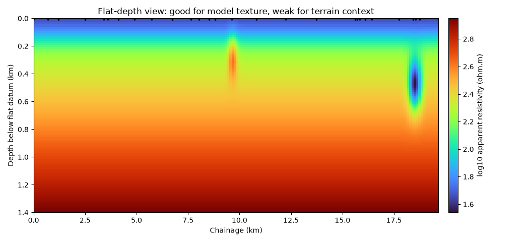
The flat panel is still useful for checking model continuity and depth trends. Its weakness is that every station appears to sit at the same datum. On a profile with more than 100 m of relief, this can make a shallow feature look laterally continuous when it is actually tied to terrain.

fig, ax = plt.subplots(figsize=(10.5, 4.8))
mesh = ax.pcolormesh(
    x_nodes, z_nodes, log10_rho, shading="auto", cmap="turbo"
)
ax.invert_yaxis()
ax.scatter(
    chain_km,
    np.zeros_like(chain_km),
    marker="v",
    s=35,
    color="black",
    zorder=4,
)
ax.set_xlabel("Chainage (km)")
ax.set_ylabel("Depth below flat datum (km)")
ax.set_title(
    "Flat-depth view: good for model texture, weak for terrain context"
)
cbar = fig.colorbar(mesh, ax=ax, pad=0.02)
cbar.set_label("log10 apparent resistivity (ohm.m)")
fig.tight_layout()

6. Terrain-following section

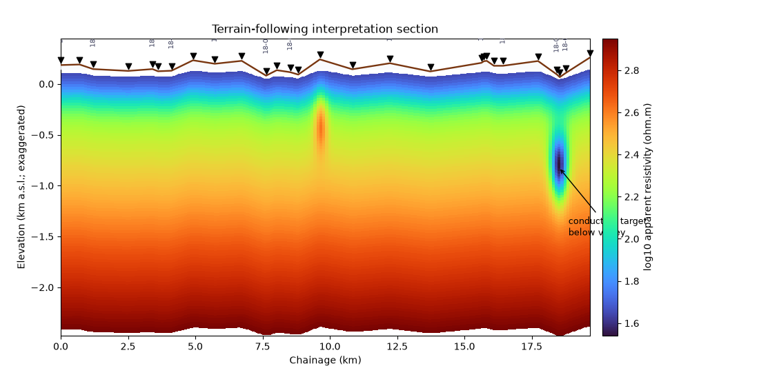
drape_section converts a depth grid into absolute elevation coordinates. draw_topo_section then masks the air above the surface and places station pins at the real terrain surface. The model values are unchanged; only the vertical coordinate system is changed.

cfg = TopoConfig(
    enabled=True,
    exaggeration=1.8,
    fill_color="#f8fafc",
    fill_alpha=0.86,
    line_color="#78350f",
    line_width=1.7,
    marker_pad_fraction=0.018,
)

x_draped, z_draped, log10_rho_draped = drape_section(
    x_nodes,
    z_nodes,
    log10_rho,
    surface_km,
    exaggeration=cfg.exaggeration,
)

fig, ax = plt.subplots(figsize=(11.0, 5.6))
mesh = ax.pcolormesh(
    x_draped, z_draped, log10_rho_draped, shading="auto", cmap="turbo"
)
draw_topo_section(ax, chain_km, elev_m, names, cfg=cfg, dark=False)

target_elev = interp_elev(
    chain_km, elev_m / 1000.0, np.array([valley_centre])
)[0]
ax.annotate(
    "conductive target\nbelow valley",
    xy=(valley_centre, target_elev - 0.48 * cfg.exaggeration),
    xytext=(valley_centre + 0.35, target_elev - 0.85 * cfg.exaggeration),
    arrowprops={"arrowstyle": "->", "color": "black", "lw": 1.0},
    fontsize=9,
    ha="left",
)

ax.set_xlabel("Chainage (km)")
ax.set_ylabel("Elevation (km a.s.l.; exaggerated)")
ax.set_title("Terrain-following interpretation section")
cbar = fig.colorbar(mesh, ax=ax, pad=0.02)
cbar.set_label("log10 apparent resistivity (ohm.m)")
fig.subplots_adjust(top=0.90, bottom=0.13, left=0.08, right=0.92)

7. Side-by-side decision panel

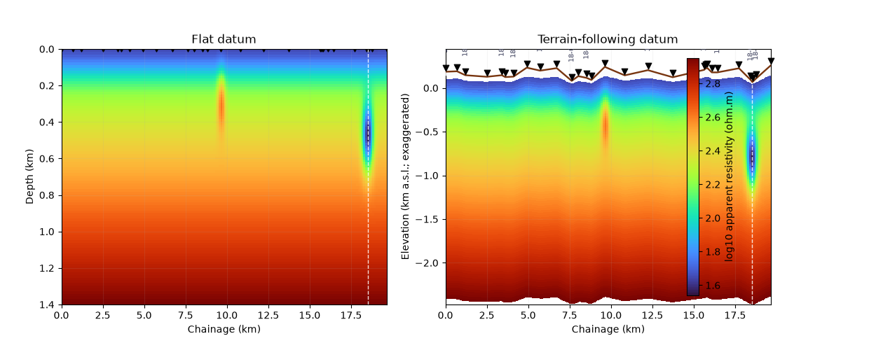
The final figure is the one you would use in a report review. It keeps the flat and topo-aware views together, so the team can separate true data/model changes from display-coordinate changes.

fig, axs = plt.subplots(1, 2, figsize=(12.5, 5.0), sharex=True)

flat = axs[0].pcolormesh(
    x_nodes, z_nodes, log10_rho, shading="auto", cmap="turbo"
)
axs[0].invert_yaxis()
axs[0].scatter(
    chain_km, np.zeros_like(chain_km), marker="v", s=25, color="black"
)
axs[0].set_title("Flat datum")
axs[0].set_xlabel("Chainage (km)")
axs[0].set_ylabel("Depth (km)")

topo = axs[1].pcolormesh(
    x_draped, z_draped, log10_rho_draped, shading="auto", cmap="turbo"
)
draw_topo_section(axs[1], chain_km, elev_m, names, cfg=cfg, dark=False)
axs[1].set_title("Terrain-following datum")
axs[1].set_xlabel("Chainage (km)")
axs[1].set_ylabel("Elevation (km a.s.l.; exaggerated)")

for ax in axs:
    ax.axvline(valley_centre, color="white", ls="--", lw=1.0, alpha=0.85)
    ax.grid(alpha=0.12)

cbar = fig.colorbar(topo, ax=axs, pad=0.02, shrink=0.88)
cbar.set_label("log10 apparent resistivity (ohm.m)")
fig.subplots_adjust(top=0.86, bottom=0.13, left=0.07, right=0.88, wspace=0.18)

8. Interpretation notes

In practice, use the topo-aware view when:

• shallow anomalies are discussed relative to station position or hillslope;

• boreholes, geology contacts, or mapped structures are plotted in elevation;

• the line crosses a ridge/valley where elevation relief is comparable to the shallow depth interval of interest;

• you compare multiple lines with different local datums.

Keep the flat-depth view available as a quality-control companion. It is often easier to spot interpolation artefacts, isolated cells, or model smoothing behaviour before the section is draped over terrain.