Run a local forward-model agent

Not every agent is about language. ForwardModelAgent runs pyCSAMT’s physics code locally: given a layered earth model it returns the synthetic magnetotelluric response — apparent resistivity and phase versus period — with no field data and no LLM involved.

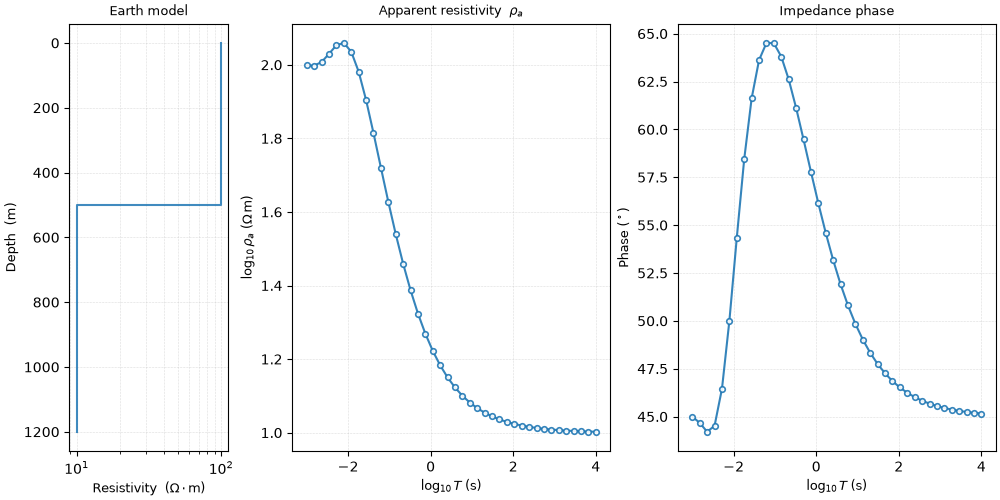
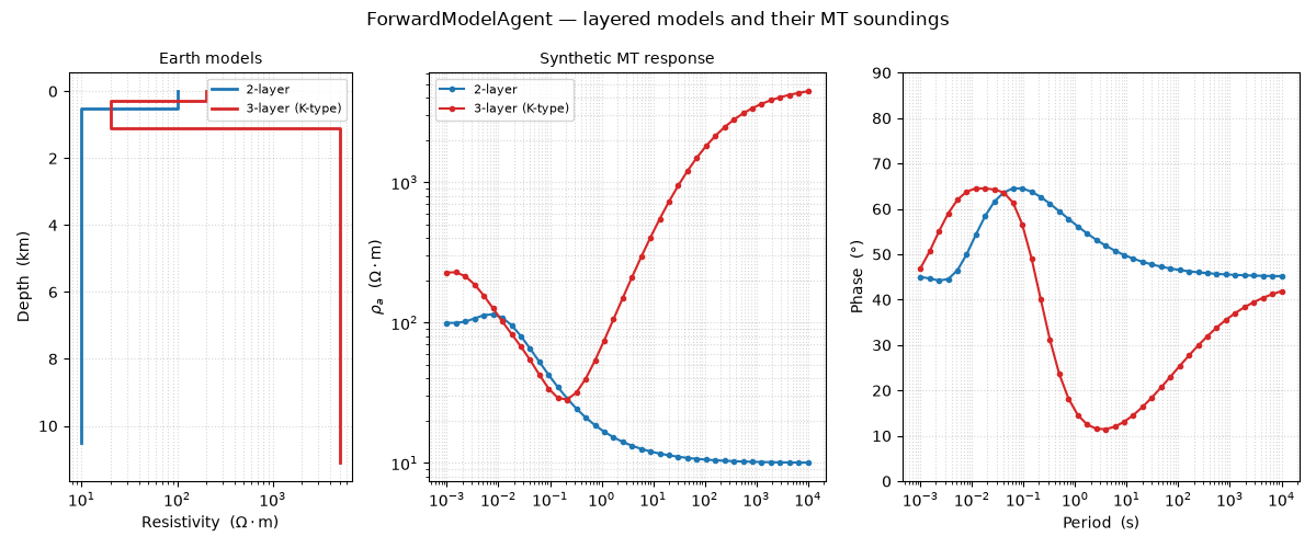
This example computes the response of a simple two-layer model, then a three-layer model with a conductive middle layer, and plots both the earth model and the sounding curve it produces.

A two-layer model

The agent takes a model dict with per-layer resistivity (Ω·m) and the thickness (m) of every layer except the terminating half-space. The result exposes the frequency grid together with rho_a and phase arrays — the classic MT sounding curve.

import numpy as np

from pycsamt.agents import ForwardModelAgent
from pycsamt.api.agents import AGENT_CONFIG

two_layer = {"resistivity": [100.0, 10.0], "thickness": [500.0]}

with AGENT_CONFIG.offline():
    res2 = ForwardModelAgent().execute({"model": two_layer})

print("status :", res2.status)
print("summary:", res2.summary)
print("n freqs:", len(res2.get("freqs")))
print(
    "rho_a range (ohm.m):",
    f"{np.min(res2.get('rho_a')):.1f} - {np.max(res2.get('rho_a')):.1f}",
)

status : success
summary: 1-D forward: 2 layers. no observed data. 1 figure(s).
n freqs: 40
rho_a range (ohm.m): 10.1 - 114.7

A three-layer model

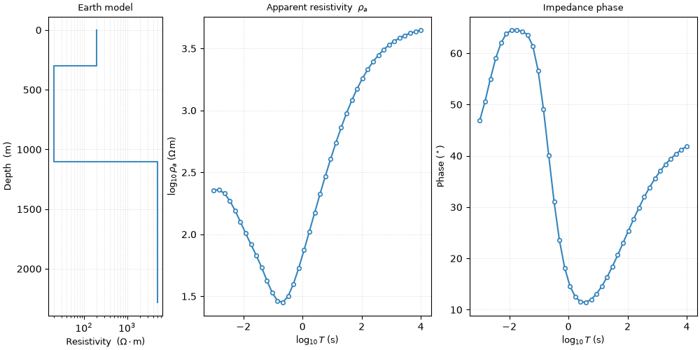
Adding a conductive middle layer (a classic “K-type” section: resistive–conductive–resistive) changes the sounding curve markedly. The same call returns the arrays for this model.

three_layer = {
    "resistivity": [200.0, 20.0, 5000.0],
    "thickness": [300.0, 800.0],
}

with AGENT_CONFIG.offline():
    res3 = ForwardModelAgent().execute({"model": three_layer})

print("status :", res3.status)
print("summary:", res3.summary)

status : success
summary: 1-D forward: 3 layers. no observed data. 1 figure(s).

Plot the model and its response

The left panel draws each earth model as a resistivity–depth staircase; the right panels overlay the two synthetic sounding curves (apparent resistivity on top, phase below) versus period. The conductive middle layer of the three-layer model pulls its apparent-resistivity curve down at intermediate periods — exactly the diagnostic signature such a layer imprints on real data.

import matplotlib.pyplot as plt


def depth_profile(model, floor_km=10.0):
    """Return (resistivity, depth) arrays that draw a layered model as steps."""
    rho = np.asarray(model["resistivity"], dtype=float)
    thick = np.asarray(model["thickness"], dtype=float)
    tops = np.concatenate([[0.0], np.cumsum(thick)])
    bottom = tops[-1] + floor_km * 1000.0  # extend the half-space
    rho_steps, depth_steps = [], []
    for i, r in enumerate(rho):
        top = tops[i]
        base = tops[i + 1] if i + 1 < len(tops) else bottom
        rho_steps += [r, r]
        depth_steps += [top, base]
    return np.array(rho_steps), np.array(depth_steps)


models = [
    ("2-layer", two_layer, res2, "#1f77b4"),
    ("3-layer (K-type)", three_layer, res3, "#d62728"),
]

fig, (ax_m, ax_r, ax_p) = plt.subplots(
    1,
    3,
    figsize=(12, 5),
    gridspec_kw={"width_ratios": [1, 1.4, 1.4]},
)

# ── earth models (resistivity vs depth) ──
for label, model, _res, color in models:
    rho_steps, depth_steps = depth_profile(model)
    ax_m.plot(rho_steps, depth_steps / 1000.0, color=color, lw=2, label=label)
ax_m.set_xscale("log")
ax_m.invert_yaxis()
ax_m.set_xlabel(r"Resistivity  ($\Omega\cdot$m)")
ax_m.set_ylabel("Depth  (km)")
ax_m.set_title("Earth models", fontsize=10)
ax_m.legend(fontsize=8)
ax_m.grid(True, which="both", ls=":", alpha=0.5)

# ── sounding curves ──
for label, _model, res, color in models:
    period = 1.0 / np.asarray(res.get("freqs"))
    ax_r.loglog(
        period, res.get("rho_a"), "-o", ms=3, color=color, label=label
    )
    ax_p.semilogx(period, res.get("phase"), "-o", ms=3, color=color)

ax_r.set_ylabel(r"$\rho_a$  ($\Omega\cdot$m)")
ax_r.set_title("Synthetic MT response", fontsize=10)
ax_r.legend(fontsize=8)
ax_r.grid(True, which="both", ls=":", alpha=0.5)

ax_p.set_ylabel("Phase  (°)")
ax_p.set_xlabel("Period  (s)")
ax_p.set_ylim(0, 90)
ax_p.grid(True, which="both", ls=":", alpha=0.5)

fig.suptitle(
    "ForwardModelAgent — layered models and their MT soundings", fontsize=12
)
fig.tight_layout()