Confidence-gated EMAP filtering

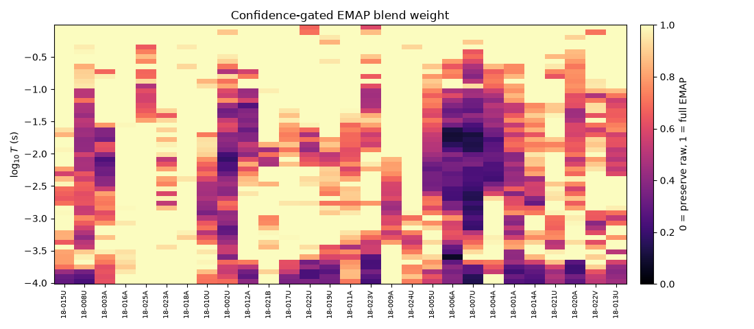
A spatial EMAP filter can stabilise a noisy station profile, but applying it everywhere with the same strength can over-smooth good data. A more robust correction is to let the confidence score control the amount of filtering:

• high-confidence rows are preserved;

• low-confidence rows are replaced by the EMAP estimate;

• marginal rows are blended between raw and filtered values.

This example uses pycsamt.emtools.confidence_gated_emap_filter() to turn EMAP from a blunt smoothing tool into an auditable correction. The result includes corrected sites, a station-level report, and a full station-frequency decision table.

1. Imports and data

import os
import sys
from pathlib import Path

import matplotlib.pyplot as plt
import numpy as np


def repo_root():
    root = os.environ.get("PYCSAMT_DOCS_REPO_ROOT")
    return Path(root) if root else Path(__file__).resolve().parents[3]


ROOT = repo_root()
if str(ROOT) not in sys.path:
    sys.path.insert(0, str(ROOT))

from _corr_data import curves, demo_line, plot_before_after

from pycsamt.emtools import (
    apply_emap_filter,
    confidence_gated_emap_filter,
    plot_emap_filter_profile,
    plot_emap_filter_psection,
)

baseline = demo_line("L18PLT")
raw_for_full = demo_line("L18PLT")
raw_for_gated = demo_line("L18PLT")

2. Full EMAP versus confidence-gated EMAP

A full EMAP filter is a useful reference: it shows the maximum correction that would be applied if we trusted the spatial smoother everywhere. The confidence-gated version starts from the same EMAP estimate but blends it row-by-row using confidence.

component = "xy"
window = 5
ci_hi = 0.90
ci_lo = 0.62

full = apply_emap_filter(
    raw_for_full,
    method="tma",
    window=window,
    component=component,
    recursive=False,
)

gated = confidence_gated_emap_filter(
    raw_for_gated,
    before_sites=baseline,
    method="tma",
    confidence_method="composite",
    component=component,
    ci_hi=ci_hi,
    ci_lo=ci_lo,
    blend_power=1.3,
    window=window,
    recursive=False,
)

print(gated.summary())
print("Gated EMAP actions:")
print(gated.decisions["action"].value_counts(dropna=False).to_string())
print("Station-level report:")
print(gated.report.head(10).to_string(index=False))

EMAPFilterResult(method='tma', confidence='composite', preserved=0, blended=801, filtered=683)
Gated EMAP actions:
action
blended     801
filtered    683
Station-level report:
station  n_freq  n_preserved  n_blended  n_filtered  mean_blend_weight  median_confidence  median_delta_log10_abs_z
18-015U      53            0         23          30           0.889395           0.604330                 -0.280786
18-008U      53            0         46           7           0.653767           0.718712                  0.209403
18-003A      53            0         31          22           0.765334           0.668071                  0.155666
18-016A      53            0          9          44           0.992540           0.588106                 -0.616073
18-025A      53            0         15          38           0.911385           0.574674                  0.242369
18-023A      53            0         18          35           0.934597           0.584983                  0.150707
18-018A      53            0          5          48           0.994388           0.586036                  0.025880
18-010U      53            0         30          23           0.822049           0.633638                 -0.299460
18-002U      53            0         48           5           0.560361           0.725523                  0.033506
18-012A      53            0         28          25           0.751624           0.644116                  0.160063

3. Where did the gated filter act?

The decision table is the audit trail. This plot shows the blend weight used at every station-frequency row. Values near 0 mean the raw data were preserved; values near 1 mean the EMAP estimate replaced the raw row.

dec = gated.decisions.copy()
stations = dec["station"].drop_duplicates().astype(str).tolist()
periods = np.sort(dec["log10_period"].dropna().unique())
blend = np.full((periods.size, len(stations)), np.nan, dtype=float)

for j, station in enumerate(stations):
    sub = dec[dec["station"].astype(str) == station]
    lookup = {
        float(row.log10_period): float(row.blend_weight)
        for _, row in sub.iterrows()
        if np.isfinite(row.log10_period)
    }
    for i, period in enumerate(periods):
        blend[i, j] = lookup.get(float(period), np.nan)

fig, ax = plt.subplots(figsize=(11.0, 4.8))
im = ax.imshow(
    blend,
    aspect="auto",
    origin="lower",
    interpolation="nearest",
    cmap="magma",
    vmin=0.0,
    vmax=1.0,
    extent=(-0.5, len(stations) - 0.5, periods.min(), periods.max()),
)
ax.set_xticks(np.arange(len(stations)))
ax.set_xticklabels(stations, rotation=90, fontsize=7)
ax.set_ylabel(r"$\log_{10}T$ (s)")
ax.set_title("Confidence-gated EMAP blend weight")
cbar = fig.colorbar(im, ax=ax, pad=0.02)
cbar.set_label("0 = preserve raw, 1 = full EMAP")
fig.tight_layout()

4. Compare survey-scale pseudo-sections

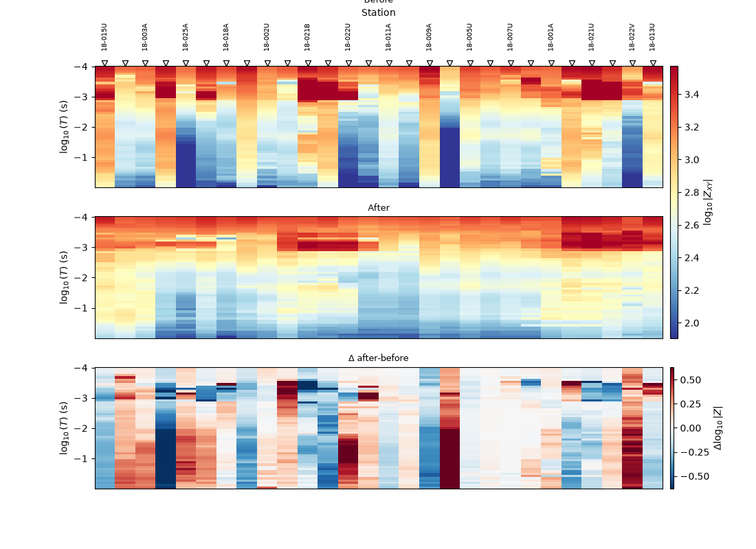
The pseudo-section summary compares raw and gated-filtered impedance. The delta panel should be structured and limited, not a blanket change across the whole survey.

plot_emap_filter_psection(
    baseline,
    gated.sites,
    method="tma",
    component=component,
    window=window,
    station_label_step=2,
    figsize=(11.0, 8.0),
)

<Figure size 1100x800 with 5 Axes>

5. Compare a target-period station profile

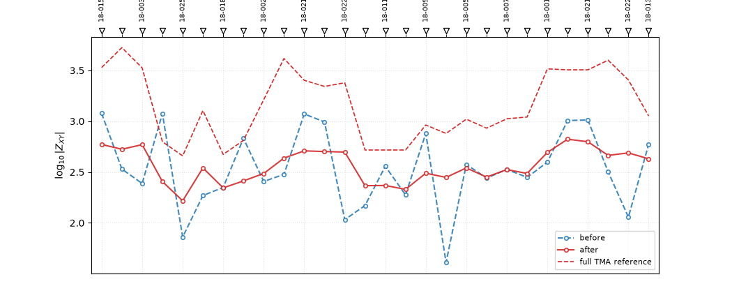
A profile at one period is often the clearest way to see over-smoothing. Here the full EMAP result is shown as a dashed reference, while the gated result follows it only where confidence demands correction.

period_s = 0.05
fig, ax = plt.subplots(figsize=(10.5, 4.4))
plot_emap_filter_profile(
    baseline,
    gated.sites,
    method="tma",
    component=component,
    period_s=period_s,
    window=window,
    ax=ax,
    station_label_step=2,
)

# Overlay full EMAP as a third profile for context.
raw = curves(baseline, quantity="rho", component=component)
full_curves = curves(full, quantity="rho", component=component)
gated_curves = curves(gated.sites, quantity="rho", component=component)
labels = list(raw)


def value_at_period(curve_map, station, period):
    periods_, values = curve_map[station]
    idx = int(np.nanargmin(np.abs(np.log10(periods_) - np.log10(period))))
    return float(np.log10(max(values[idx], 1e-24)))


x = np.arange(len(labels))
full_vals = [value_at_period(full_curves, st, period_s) for st in labels]
ax.plot(
    x,
    full_vals,
    "--",
    lw=1.2,
    color="#dc2626",
    label="full TMA reference",
)
ax.legend(fontsize=8)
ax.set_title(f"Confidence-gated EMAP at T={period_s:g} s")

Text(0.5, 1.247769906860816, 'Confidence-gated EMAP at T=0.05 s')

6. Sounding-level sanity check

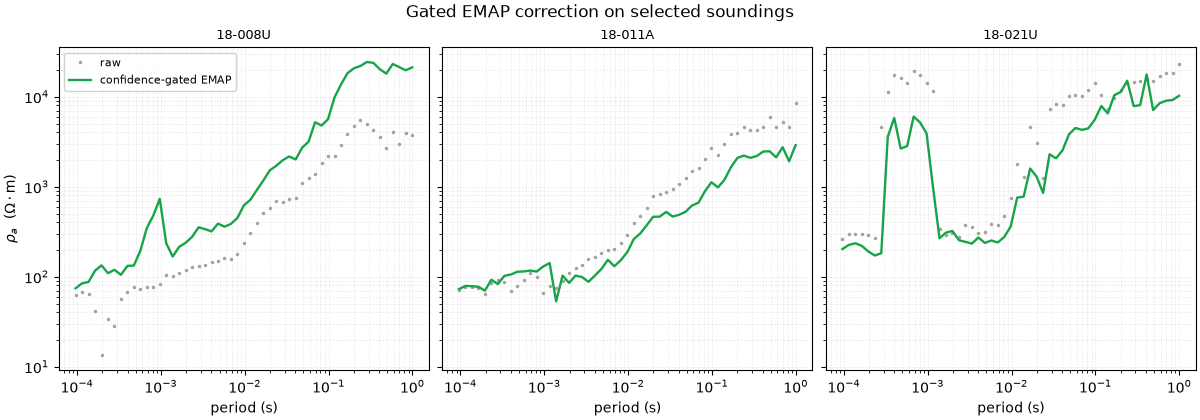
A final curve overlay confirms that the gated filter does not rewrite the whole sounding. It should mainly stabilise problematic frequency rows while preserving high-confidence curve shape.

pick = [labels[1], labels[len(labels) // 2], labels[-4]]

plot_before_after(
    raw,
    gated_curves,
    pick,
    quantity="rho",
    labels=("raw", "confidence-gated EMAP"),
    colors=("#a8a29e", "#16a34a"),
    title="Gated EMAP correction on selected soundings",
)

<Figure size 1200x420 with 3 Axes>

7. Decision guide

Prefer confidence-gated EMAP when the line has mostly good data with localized station-frequency problems. Prefer a full EMAP pass only when the whole profile is noisy or when the processing objective is a deliberately smoothed regional trend. Always keep the decision table: it records which rows were preserved, blended, or filtered.