
Note
Go to the end to download the full example code.
Reviewer-response audit for conditioned AMT/MT data#
Peer review often asks for more than a clean final pseudo-section. Reviewers may ask how confidence scores were defined, whether low-quality frequencies were interpolated or rejected, how electromagnetic interference was handled, which adaptive moving-average parameters were used, whether 2-D inversion is defensible, and whether galvanic distortion was checked.
This case study shows how to answer those questions with reproducible tables and figures instead of prose alone. It is written as a general field-data audit template:
replace the two WILLY example paths with your own EDI folders;
keep the same report tables as an audit trail;
include the generated figures in a manuscript response, thesis appendix, or processing notebook.
The example uses the bundled WILLY L18PLT and L22PLT lines because
they are small enough for the gallery while still behaving like real survey
lines.
1. Imports, paths, and audit policy#
The output directory is deliberately local to the example gallery. It is ignored by git, so the generated CSV and PNG files can be inspected or copied without becoming source files.
from __future__ import annotations

import os
import sys
from pathlib import Path

import matplotlib.pyplot as plt
import numpy as np
import pandas as pd

try:
    EXAMPLE_DIR = Path(__file__).resolve().parent
except NameError:
    EXAMPLE_DIR = Path.cwd()


def repo_root() -> Path:
    root = os.environ.get("PYCSAMT_DOCS_REPO_ROOT")
    return Path(root) if root else EXAMPLE_DIR.parents[2]


ROOT = repo_root()
if str(ROOT) not in sys.path:
    sys.path.insert(0, str(ROOT))
if str(EXAMPLE_DIR) not in sys.path:
    sys.path.insert(0, str(EXAMPLE_DIR))

from pycsamt.emtools import (  # noqa: E402
    confidence_gated_emap_filter,
    correct_ss_ama,
    edit_frequencies_by_confidence,
    emi_mitigation_report,
    ensure_sites,
    estimate_ss_ama,
    frequency_confidence_table,
    groom_bailey_table,
    plot_confidence_band_summary,
    plot_confidence_profile,
    plot_frequency_confidence_psection,
    plot_skew_traffic_psection,
    plot_ss_delta_profile,
    plot_strike_profile,
    pre2d_inversion_assessment,
    qc_flags,
    station_confidence_table,
)
from pycsamt.emtools.remove_noise import snr_table  # noqa: E402

LINES = {
    "L18PLT": ROOT / "data" / "AMT" / "WILLY_DATA" / "L18PLT",
    "L22PLT": ROOT / "data" / "AMT" / "WILLY_DATA" / "L22PLT",
}

OUT = EXAMPLE_DIR / "workspaces" / "reviewer_response_audit"
OUT.mkdir(parents=True, exist_ok=True)

CI_HI = 0.95
CI_LO = 0.85
MAIN_HZ = 50.0
STATIC_SHIFT_WINDOWS = (1, 2, 3, 4)
2. Mathematical definitions used in the audit#
The confidence ratio is a finite-score weighted mean:
s_k are diagnostic scores, w_k are their weights, and I_k is
one only when a score is finite. In this workflow the default pyCSAMT
scores are coverage, tensor uncertainty, off-diagonal consistency, diagonal
leakage, phase smoothness, and spatial coherence. The review classes are:
The adaptive moving-average static-shift estimate uses determinant apparent resistivity
For station i, the log-resistivity deviation from a neighboring spatial
trend is reduced to Delta_i and applied as
Power-line harmonics are documented by the frequency rule
Groom–Bailey-style galvanic-distortion diagnostics fit
with real, frequency-independent distortion matrix D.
def write_table(table, path: Path) -> pd.DataFrame:
    """Write a DataFrame-like object and return a plain DataFrame."""
    df = getattr(table, "df", table)
    if not isinstance(df, pd.DataFrame):
        df = pd.DataFrame(df)
    df.to_csv(path, index=False)
    return df


def save_current_figure(path: Path) -> None:
    """Save the current gallery figure to the audit workspace."""
    fig = plt.gcf()
    fig.savefig(path, dpi=180, bbox_inches="tight")
3. Load each line and create the core audit tables#
These CSV files are the part most useful to a student facing similar reviewer comments. They show what was calculated, which rows were edited, and what limitations remain.
sites_by_line = {}
summary_rows = []

for line, edi_dir in LINES.items():
    line_out = OUT / line
    line_out.mkdir(parents=True, exist_ok=True)

    sites = ensure_sites(str(edi_dir), recursive=False, verbose=0)
    sites_by_line[line] = sites

    freq_conf = write_table(
        frequency_confidence_table(
            sites,
            method="composite",
            ci_hi=CI_HI,
            ci_lo=CI_LO,
        ),
        line_out / "frequency_confidence.csv",
    )
    write_table(
        station_confidence_table(
            sites,
            method="composite",
        ),
        line_out / "station_confidence.csv",
    )
    write_table(qc_flags(sites), line_out / "qc_flags.csv")
    write_table(snr_table(sites), line_out / "snr_table.csv")
    write_table(
        emi_mitigation_report(
            sites,
            remote_reference_attempted=False,
            remote_reference_reason=(
                "The bundled gallery EDIs do not include remote-reference "
                "time series. This audit documents transfer-function-level "
                "mitigation and diagnostics."
            ),
            mains_hz=MAIN_HZ,
        ),
        line_out / "emi_mitigation_report.csv",
    )

    edited = edit_frequencies_by_confidence(
        sites,
        mode="recover",
        before_sites=sites,
        ci_hi=CI_HI,
        ci_lo=CI_LO,
        reject="mask",
        interpolation="linear",
    )
    write_table(edited.report, line_out / "frequency_edit_report.csv")
    write_table(edited.decisions, line_out / "frequency_edit_decisions.csv")

    emap = confidence_gated_emap_filter(
        sites,
        before_sites=sites,
        method="flma",
        confidence_method="composite",
        component="xy",
        ci_hi=CI_HI,
        ci_lo=CI_LO,
        window=5,
    )
    write_table(emap.report, line_out / "confidence_gated_emap_report.csv")
    write_table(
        emap.decisions, line_out / "confidence_gated_emap_decisions.csv"
    )

    safe = int((freq_conf["confidence"] >= CI_HI).sum())
    recoverable = int(
        (
            (freq_conf["confidence"] >= CI_LO)
            & (freq_conf["confidence"] < CI_HI)
        ).sum()
    )
    reject = int((freq_conf["confidence"] < CI_LO).sum())
    summary_rows.append(
        {
            "line": line,
            "stations": len(station_confidence_table(sites)),
            "frequency_rows": len(freq_conf),
            "safe_rows": safe,
            "recoverable_rows": recoverable,
            "reject_rows": reject,
            "emap_preserved": emap.n_preserved,
            "emap_blended": emap.n_blended,
            "emap_filtered": emap.n_filtered,
        }
    )

summary = pd.DataFrame(summary_rows)
summary.to_csv(OUT / "all_lines_summary.csv", index=False)
print(summary.to_string(index=False))
  line  stations  frequency_rows  safe_rows  recoverable_rows  reject_rows  emap_preserved  emap_blended  emap_filtered
L18PLT        28            1484          0                 5         1479               0             5           1479
L22PLT        25            1325          0                39         1286               0            39           1286
4. Confidence figures: justify preserve/recover/reject decisions#
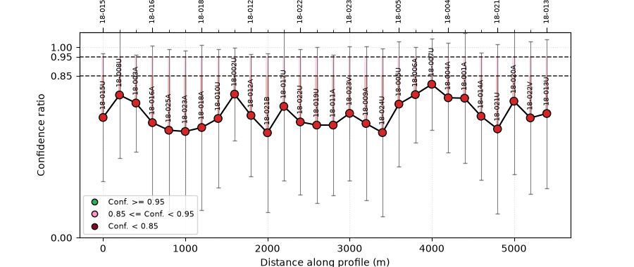
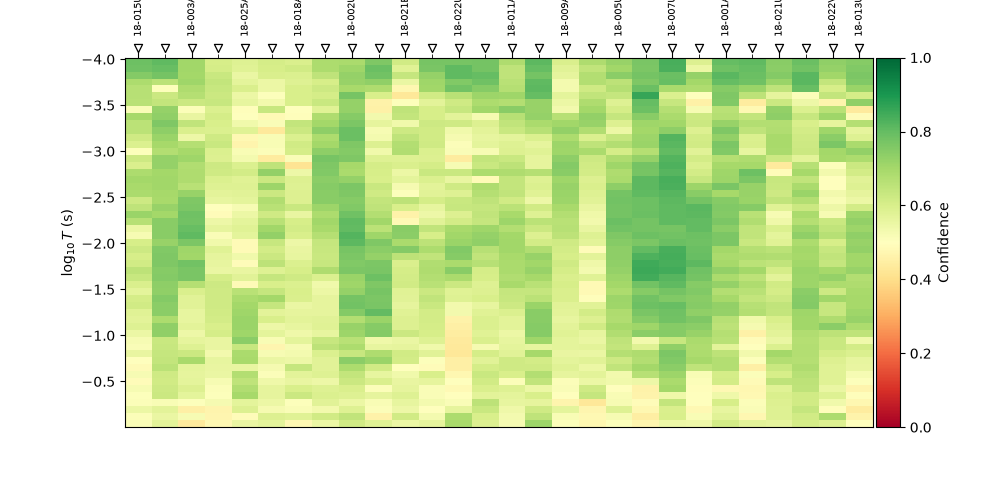
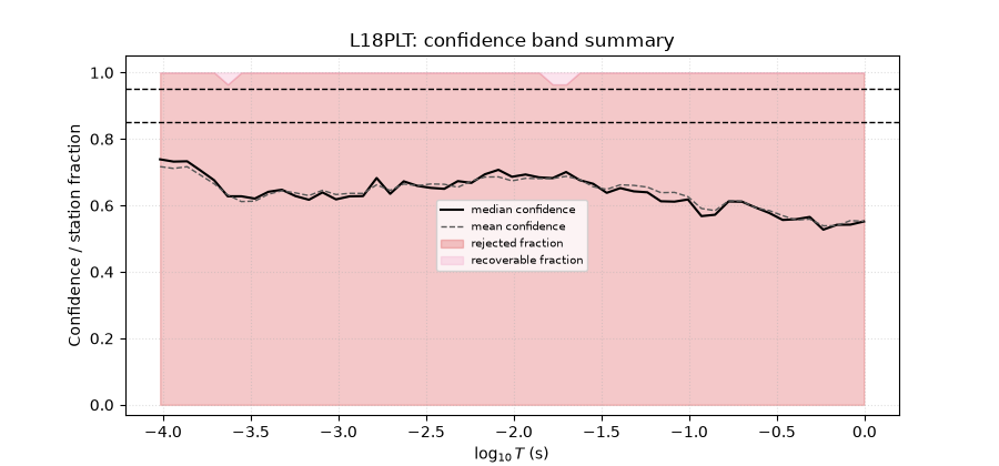
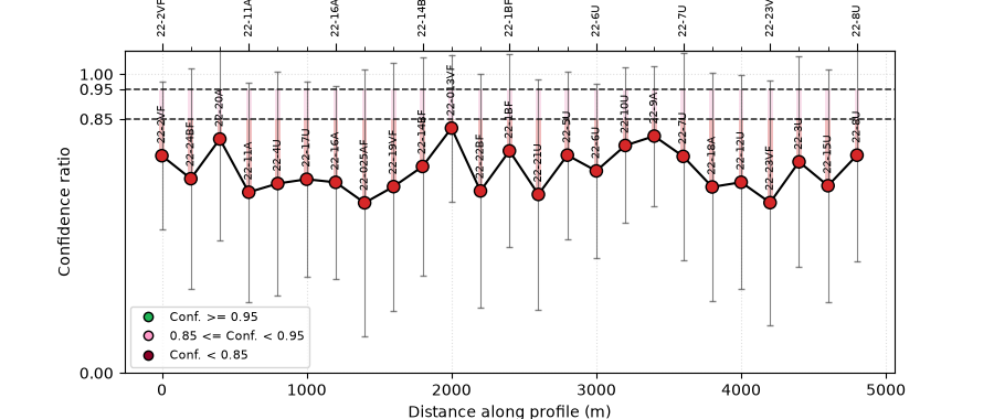
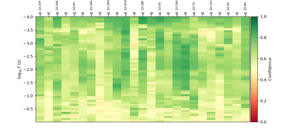
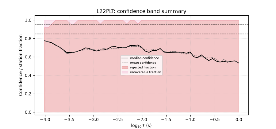
These plots answer the common request: “show where the confidence classes occur, not only the final smoothed response.” The first figure is a station profile; the second is a station-period confidence pseudo-section; the third summarizes the confidence bands.
for line, sites in sites_by_line.items():
    fig_dir = OUT / line / "figures"
    fig_dir.mkdir(exist_ok=True)

    ax = plot_confidence_profile(
        sites,
        method="composite",
        ci_hi=CI_HI,
        ci_lo=CI_LO,
        figsize=(9.0, 3.8),
    )
    ax.set_title(f"{line}: station confidence profile")
    save_current_figure(fig_dir / "confidence_profile.png")

    ax = plot_frequency_confidence_psection(
        sites,
        method="composite",
        ci_hi=CI_HI,
        ci_lo=CI_LO,
        figsize=(10.0, 4.8),
    )
    ax.set_title(f"{line}: frequency-confidence pseudo-section")
    save_current_figure(fig_dir / "frequency_confidence_psection.png")

    ax = plot_confidence_band_summary(
        sites,
        method="composite",
        ci_hi=CI_HI,
        ci_lo=CI_LO,
        figsize=(9.0, 4.2),
    )
    ax.set_title(f"{line}: confidence band summary")
    save_current_figure(fig_dir / "confidence_band_summary.png")
5. EMI and frequency-edit evidence#
The tables above document remote-reference status, power-line harmonic counts, station-level SNR, and edit decisions. A compact reviewer response can cite these tables directly and state that recovered frequencies remain flagged by the decision table rather than being treated as independent measurements.
for line in LINES:
    line_out = OUT / line
    emi = pd.read_csv(line_out / "emi_mitigation_report.csv")
    edit = pd.read_csv(line_out / "frequency_edit_report.csv")
    print(f"\n{line}: EMI and edit summary")
    print(
        emi[
            [
                "station",
                "remote_reference_attempted",
                "harmonic_z_samples",
                "applied_measures",
            ]
        ]
        .head(5)
        .to_string(index=False)
    )
    print(
        edit[
            [
                "station",
                "n_freq_before",
                "n_freq_after",
                "confidence_median_before",
                "confidence_median_after",
            ]
        ]
        .head(5)
        .to_string(index=False)
    )
L18PLT: EMI and edit summary
station  remote_reference_attempted  harmonic_z_samples                                                                                                                                                                                             applied_measures
18-001A                       False                   0 notch_powerline(mode=interp, mains_hz=50, n_harm=30, tol_hz=0.08); mask_incoherent_freqs / frequency_confidence_table as needed; hampel_filter_freq / spatial_median_filter / rpca_offdiag_denoise as needed
18-002U                       False                   0 notch_powerline(mode=interp, mains_hz=50, n_harm=30, tol_hz=0.08); mask_incoherent_freqs / frequency_confidence_table as needed; hampel_filter_freq / spatial_median_filter / rpca_offdiag_denoise as needed
18-003A                       False                   0 notch_powerline(mode=interp, mains_hz=50, n_harm=30, tol_hz=0.08); mask_incoherent_freqs / frequency_confidence_table as needed; hampel_filter_freq / spatial_median_filter / rpca_offdiag_denoise as needed
18-004A                       False                   0 notch_powerline(mode=interp, mains_hz=50, n_harm=30, tol_hz=0.08); mask_incoherent_freqs / frequency_confidence_table as needed; hampel_filter_freq / spatial_median_filter / rpca_offdiag_denoise as needed
18-005U                       False                   0 notch_powerline(mode=interp, mains_hz=50, n_harm=30, tol_hz=0.08); mask_incoherent_freqs / frequency_confidence_table as needed; hampel_filter_freq / spatial_median_filter / rpca_offdiag_denoise as needed
station  n_freq_before  n_freq_after  confidence_median_before  confidence_median_after
18-001A             53            53                  0.711753                      0.0
18-002U             53            53                  0.749480                      0.0
18-003A             53            53                  0.666613                      0.0
18-004A             53            53                  0.735994                      0.0
18-005U             53            53                  0.728841                      0.0

L22PLT: EMI and edit summary
station  remote_reference_attempted  harmonic_z_samples                                                                                                                                                                                             applied_measures
 22-1BF                       False                   0 notch_powerline(mode=interp, mains_hz=50, n_harm=30, tol_hz=0.08); mask_incoherent_freqs / frequency_confidence_table as needed; hampel_filter_freq / spatial_median_filter / rpca_offdiag_denoise as needed
 22-2VF                       False                   0 notch_powerline(mode=interp, mains_hz=50, n_harm=30, tol_hz=0.08); mask_incoherent_freqs / frequency_confidence_table as needed; hampel_filter_freq / spatial_median_filter / rpca_offdiag_denoise as needed
  22-3U                       False                   0 notch_powerline(mode=interp, mains_hz=50, n_harm=30, tol_hz=0.08); mask_incoherent_freqs / frequency_confidence_table as needed; hampel_filter_freq / spatial_median_filter / rpca_offdiag_denoise as needed
  22-4U                       False                   0 notch_powerline(mode=interp, mains_hz=50, n_harm=30, tol_hz=0.08); mask_incoherent_freqs / frequency_confidence_table as needed; hampel_filter_freq / spatial_median_filter / rpca_offdiag_denoise as needed
  22-5U                       False                   0 notch_powerline(mode=interp, mains_hz=50, n_harm=30, tol_hz=0.08); mask_incoherent_freqs / frequency_confidence_table as needed; hampel_filter_freq / spatial_median_filter / rpca_offdiag_denoise as needed
 station  n_freq_before  n_freq_after  confidence_median_before  confidence_median_after
22-013VF             53            53                  0.812743                      0.0
22-025AF             53            53                  0.629359                      0.0
  22-10U             53            53                  0.768336                      0.0
  22-11A             53            53                  0.640670                      0.0
  22-12U             53            53                  0.652714                      0.0
6. Static-shift sensitivity: show that AMA parameters were checked#
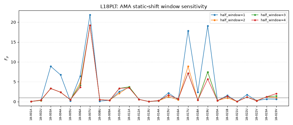
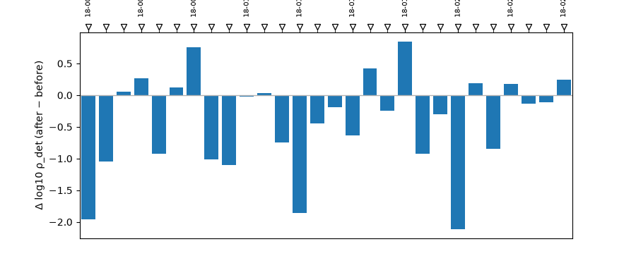
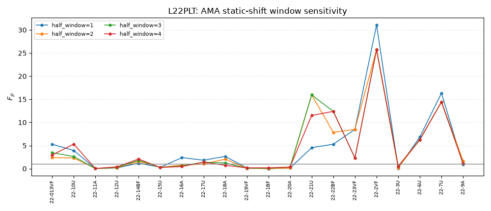
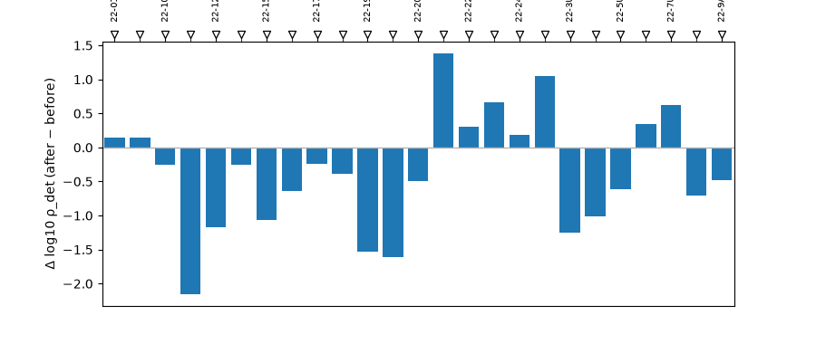
The reviewer does not only need the final static-shift correction; they need to know whether the moving-average window suppresses real geology. Here we run several neighbor windows and write a long-form sensitivity table. A stable correction should not change wildly as the window is perturbed.
for line, sites in sites_by_line.items():
    rows = []
    for half_window in STATIC_SHIFT_WINDOWS:
        factors = write_table(
            estimate_ss_ama(
                sites,
                sort_by="lon",
                half_window=half_window,
                weights="tri",
                max_skew=6.0,
            ),
            OUT / line / f"ss_ama_factors_half_window_{half_window}.csv",
        )
        for _, row in factors.iterrows():
            rows.append(
                {
                    "line": line,
                    "half_window": half_window,
                    "station": row.get("station"),
                    "delta_log10_rho": row.get("delta_log10_rho"),
                    "fac_rho": row.get("fac_rho"),
                    "fac_z": row.get("fac_z"),
                    "n_used": row.get("n_used"),
                }
            )
    sensitivity = pd.DataFrame(rows)
    sensitivity.to_csv(
        OUT / line / "ss_ama_window_sensitivity.csv", index=False
    )

    fig, ax = plt.subplots(figsize=(10.0, 4.3))
    for half_window, sub in sensitivity.groupby("half_window"):
        sub = sub.sort_values("station")
        ax.plot(
            np.arange(len(sub)),
            sub["fac_rho"].to_numpy(dtype=float),
            marker="o",
            ms=3.5,
            lw=1.2,
            label=f"half_window={half_window}",
        )
    ax.axhline(1.0, color="0.5", lw=1.0)
    labels = sensitivity[
        sensitivity["half_window"] == STATIC_SHIFT_WINDOWS[0]
    ]["station"].astype(str)
    ax.set_xticks(np.arange(len(labels)))
    ax.set_xticklabels(labels, rotation=90, fontsize=7)
    ax.set_ylabel(r"$F_\rho$")
    ax.set_title(f"{line}: AMA static-shift window sensitivity")
    ax.grid(True, axis="y", ls=":", alpha=0.5)
    ax.legend(fontsize=8, ncol=2)
    fig.tight_layout()
    save_current_figure(
        OUT / line / "figures" / "ss_ama_window_sensitivity.png"
    )

    corrected = correct_ss_ama(
        sites,
        sort_by="lon",
        half_window=3,
        weights="tri",
        max_skew=6.0,
        inplace=False,
    )
    ax = plot_ss_delta_profile(sites, corrected, figsize=(9.0, 3.8))
    ax.set_title(f"{line}: applied static-shift delta profile")
    save_current_figure(OUT / line / "figures" / "ss_delta_profile.png")
7. Dimensionality, strike, and rotation readiness#
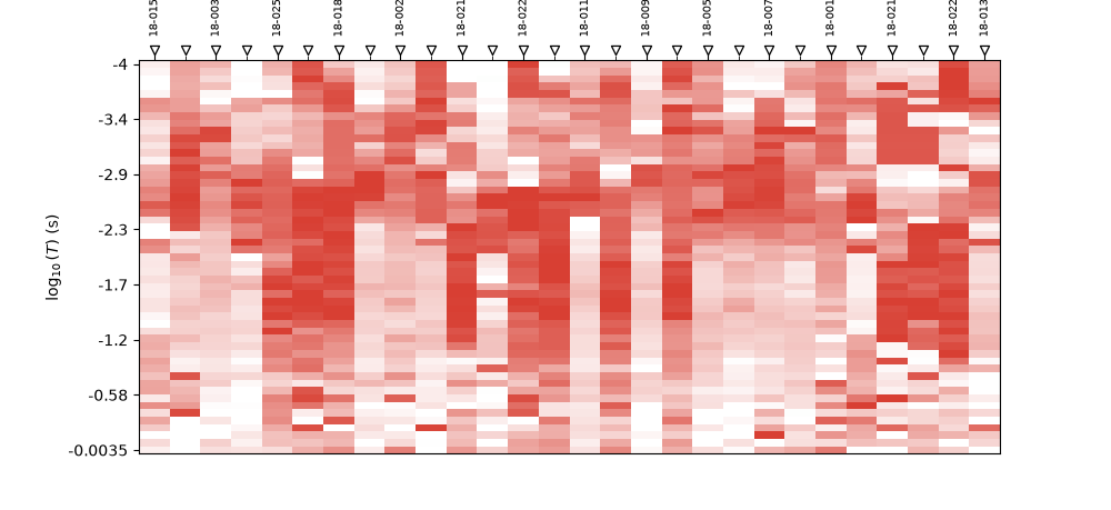
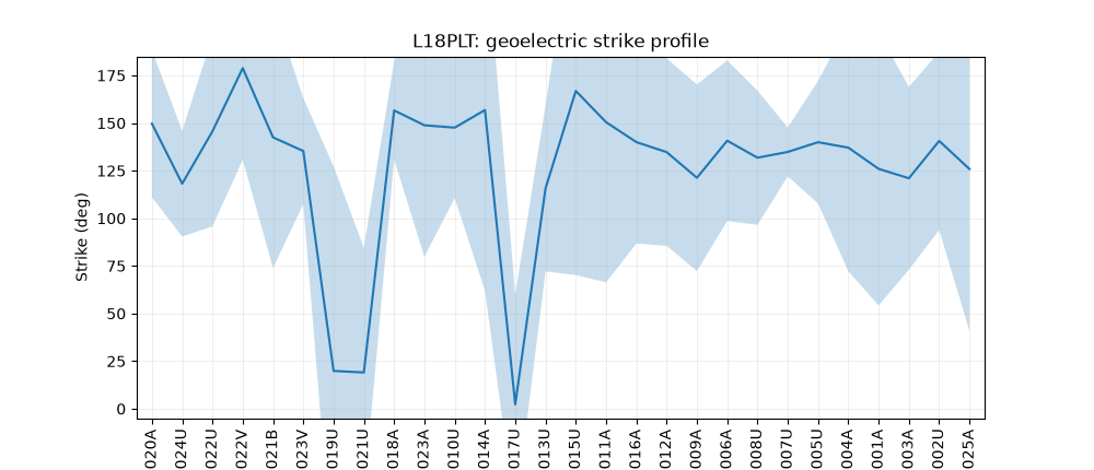
This table answers several reviewer questions at once: how much of the data is 1-D/2-D/3-D, where high skew appears, what strike estimate is obtained, and whether rotation/Groom–Bailey status was documented.
for line, sites in sites_by_line.items():
    gb = write_table(
        groom_bailey_table(sites, min_freq=4, robust=True),
        OUT / line / "groom_bailey_table.csv",
    )
    gb_ok = bool((gb.get("status", pd.Series(dtype=str)) == "ok").any())
    assessment = write_table(
        pre2d_inversion_assessment(
            sites,
            rotation_applied=False,
            groom_bailey_attempted=True,
            groom_bailey_applied=False,
            groom_bailey_reason=(
                "Groom-Bailey table was computed as a diagnostic. "
                "Correction was not applied in this gallery audit; "
                f"valid station fits present: {gb_ok}."
            ),
        ),
        OUT / line / "pre2d_inversion_assessment.csv",
    )
    print(f"\n{line}: pre-2D assessment")
    print(
        assessment[
            [
                "station",
                "frac_2d",
                "frac_3d",
                "beta_abs_p95",
                "strike_consensus_deg",
                "strike_consensus_iqr_deg",
                "recommendation",
            ]
        ]
        .head(8)
        .to_string(index=False)
    )

    ax = plot_skew_traffic_psection(sites, figsize=(10.0, 4.6))
    ax.set_title(f"{line}: skew traffic pseudo-section")
    save_current_figure(OUT / line / "figures" / "skew_traffic_psection.png")

    ax = plot_strike_profile(sites, figsize=(10.0, 4.3))
    ax.set_title(f"{line}: geoelectric strike profile")
    save_current_figure(OUT / line / "figures" / "strike_profile.png")
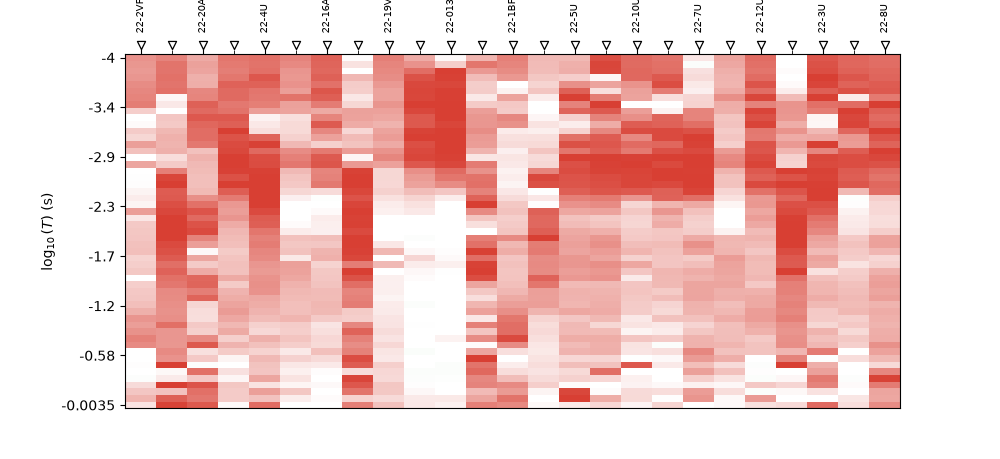
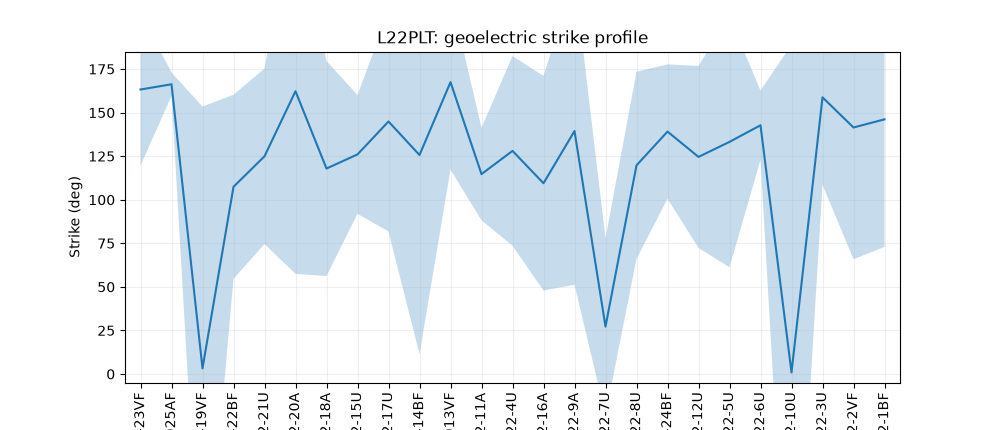
L18PLT: pre-2D assessment
station  frac_2d  frac_3d  beta_abs_p95  strike_consensus_deg  strike_consensus_iqr_deg              recommendation
18-001A 0.301887 0.660377     71.552395            -54.035882                143.487238 review_3d_effects_before_2d
18-002U 0.132075 0.754717     28.058262            -39.378789                 93.664883 review_3d_effects_before_2d
18-003A 0.075472 0.905660     41.944383            -58.974641                 95.996655 review_3d_effects_before_2d
18-004A 0.132075 0.811321     28.932956            -42.904847                129.885148 review_3d_effects_before_2d
18-005U 0.207547 0.773585     31.780380            -40.046024                 64.389509 review_3d_effects_before_2d
18-006A 0.094340 0.792453     29.351174            -39.254078                 84.350133 review_3d_effects_before_2d
18-007U 0.075472 0.849057     24.342916            -45.151003                 25.651968 review_3d_effects_before_2d
18-008U 0.132075 0.830189     49.588863            -48.187398                 70.520137 review_3d_effects_before_2d

L22PLT: pre-2D assessment
station  frac_2d  frac_3d  beta_abs_p95  strike_consensus_deg  strike_consensus_iqr_deg              recommendation
 22-1BF 0.264151 0.603774     48.305704            -33.881118                146.388871 review_3d_effects_before_2d
 22-2VF 0.264151 0.452830     29.893335            -38.551223                151.149412 unstable_strike_review_band
  22-3U 0.132075 0.867925     40.856752            -21.242391                100.424142 review_3d_effects_before_2d
  22-4U 0.226415 0.716981     41.500103            -51.972023                108.875681 review_3d_effects_before_2d
  22-5U 0.075472 0.754717     26.460833            -46.801929                143.955080 review_3d_effects_before_2d
  22-6U 0.094340 0.754717     27.302651            -37.264253                 39.823857 review_3d_effects_before_2d
  22-7U 0.075472 0.641509     30.669563             27.181654                101.511862 review_3d_effects_before_2d
  22-8U 0.132075 0.679245     30.684113            -60.279986                107.447109 review_3d_effects_before_2d
8. Groom–Bailey distortion diagnostics#
If Groom–Bailey correction is not applied, the response should still say whether it was considered. The diagnostic table records fitted status, distortion parameters, and diagonal leakage before/after the fitted correction. Do not blindly apply this correction; inspect accepted station fits first.
for line in LINES:
    gb = pd.read_csv(OUT / line / "groom_bailey_table.csv")
    cols = [
        "station",
        "status",
        "n_freq",
        "twist_deg",
        "shear_angle_deg",
        "anisotropy",
        "diagonal_ratio_before",
        "diagonal_ratio_after",
    ]
    present = [col for col in cols if col in gb.columns]
    print(f"\n{line}: Groom-Bailey diagnostic rows")
    print(gb[present].head(8).to_string(index=False))
L18PLT: Groom-Bailey diagnostic rows
station status  n_freq  twist_deg  shear_angle_deg  anisotropy  diagonal_ratio_before  diagonal_ratio_after
18-001A     ok      53   9.617139       -27.411059    0.075566               0.543368              0.246856
18-002U     ok      53   6.842063       -11.599039    0.017068               0.343245              0.231721
18-003A     ok      53   0.620507         0.774234   -0.000075               0.288563              0.286055
18-004A     ok      53  12.074518        -5.753771    0.017266               0.421292              0.279321
18-005U     ok      53   1.210542       -14.137002    0.003583               0.347065              0.263442
18-006A     ok      53   7.114697        11.414315   -0.020614               0.370648              0.221286
18-007U     ok      53   7.173695       -11.102871    0.017671               0.337301              0.232125
18-008U     ok      53  14.116591       -25.005996    0.080433               0.510774              0.221079

L22PLT: Groom-Bailey diagnostic rows
station status  n_freq  twist_deg  shear_angle_deg  anisotropy  diagonal_ratio_before  diagonal_ratio_after
 22-1BF     ok      53   4.374708        -6.792731    0.011439               0.425072              0.334408
 22-2VF     ok      53   8.389544         6.272396   -0.018317               0.266486              0.246382
  22-3U     ok      53   8.726891       -11.284760    0.027086               0.256834              0.200349
  22-4U     ok      53  -2.095210        11.997358    0.005700               0.291471              0.194229
  22-5U     ok      53   1.514622         6.438545   -0.002953               0.255549              0.211833
  22-6U     ok      53  -5.787005         8.878100    0.015633               0.246787              0.209040
  22-7U     ok      53   3.573551         1.220089   -0.001287               0.231149              0.193090
  22-8U     ok      53  -0.828289        13.929391    0.004703               0.299655              0.142907
9. What to copy into a report#
The generated workspace now contains both human-readable figures and machine-readable CSV files. A concise response to a reviewer can cite:
frequency_confidence.csvand confidence figures for CR definition and preserve/recover/reject classes;frequency_edit_decisions.csvandfrequency_edit_report.csvfor the treatment of reconstructed or masked frequencies;emi_mitigation_report.csvandsnr_table.csvfor interference documentation;ss_ama_window_sensitivity.csvand static-shift figures for moving average parameter sensitivity;pre2d_inversion_assessment.csvfor dimensionality, skew, strike, and rotation readiness;groom_bailey_table.csvfor galvanic-distortion diagnostics.
To use this example with a new survey, replace LINES near the top with
paths to the student’s EDI folders. The rest of the workflow can remain the
same unless the project uses different confidence thresholds, power-line
frequency, or inversion period band.
print(f"\nAudit workspace written to:\n{OUT}")
Audit workspace written to:
/opt/build/repo/docs/examples/corrections/workspaces/reviewer_response_audit
Total running time of the script: (0 minutes 20.745 seconds)