Confidence-gated frequency editing

Many correction failures begin before the correction itself: bad or marginal frequency rows are allowed to survive into static-shift, smoothing, rotation, or inversion. A robust workflow therefore treats frequency editing as a correction decision, not as a manual clean-up step.

This example uses pyCSAMT’s confidence editing workflow to classify every station-frequency row as kept or dropped. It then compares two correction policies:

• permissive drop removes only clearly rejected rows;

• conservative drop removes rejected and weakly marginal rows.

The point is not that one policy is always better. The point is to make the trade-off visible: permissive editing preserves more data, while conservative editing gives inversion and correction tools fewer questionable rows.

1. Imports and data

import os
import sys
from pathlib import Path

import matplotlib.pyplot as plt
import numpy as np


def repo_root():
    root = os.environ.get("PYCSAMT_DOCS_REPO_ROOT")
    return Path(root) if root else Path(__file__).resolve().parents[3]


ROOT = repo_root()
if str(ROOT) not in sys.path:
    sys.path.insert(0, str(ROOT))

from _corr_data import demo_line

from pycsamt.emtools import (
    edit_frequencies_by_confidence,
    frequency_confidence_table,
    plot_frequency_edit_decisions,
    plot_frequency_edit_summary,
)
from pycsamt.emtools._core import _get_z_block, _iter_items, _name

raw_for_permissive = demo_line("L18PLT")
raw_for_conservative = demo_line("L18PLT")
baseline = demo_line("L18PLT")

2. Inspect confidence before editing

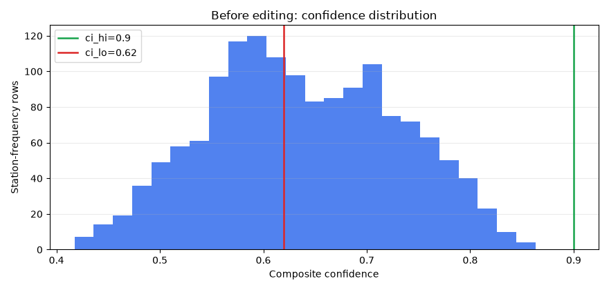
The confidence table is a station-frequency table. Rows above ci_hi are safe, rows between ci_lo and ci_hi are recoverable/marginal, and rows below ci_lo are rejected. Keeping the thresholds explicit makes later plots and reports reproducible.

ci_hi = 0.90
ci_lo = 0.62
permissive_threshold = ci_lo
conservative_threshold = 0.72

confidence = frequency_confidence_table(
    baseline,
    method="composite",
    ci_hi=ci_hi,
    ci_lo=ci_lo,
    recursive=False,
)

print("Confidence table columns:")
print(list(confidence.columns))
print(
    "Confidence range: "
    f"{confidence['confidence'].min():.3f}-"
    f"{confidence['confidence'].max():.3f}"
)
print("Confidence classes:")
confidence_values = confidence["confidence"].to_numpy(dtype=float)
confidence_class = np.where(
    confidence_values >= ci_hi,
    "safe",
    np.where(confidence_values >= ci_lo, "recoverable", "reject"),
)
unique, counts = np.unique(confidence_class, return_counts=True)
for label, count in zip(unique, counts):
    print(f"{label}: {count}")

fig, ax = plt.subplots(figsize=(8.8, 4.2))
ax.hist(
    confidence["confidence"].to_numpy(dtype=float),
    bins=24,
    color="#2563eb",
    alpha=0.80,
)
ax.axvline(ci_hi, color="#16a34a", lw=1.8, label=f"ci_hi={ci_hi}")
ax.axvline(ci_lo, color="#dc2626", lw=1.8, label=f"ci_lo={ci_lo}")
ax.set_xlabel("Composite confidence")
ax.set_ylabel("Station-frequency rows")
ax.set_title("Before editing: confidence distribution")
ax.grid(axis="y", alpha=0.25)
ax.legend()
fig.tight_layout()

Confidence table columns:
['station', 'station_index', 'distance_m', 'frequency_hz', 'period_s', 'log10_period', 'confidence', 'confidence_err', 'method', 'n_components', 'coverage', 'uncertainty', 'offdiag', 'diagonal', 'phase', 'spatial', 'logrho_proxy', 'flags']
Confidence range: 0.417-0.863
Confidence classes:
recoverable: 801
reject: 683

3. Policy A: permissive drop

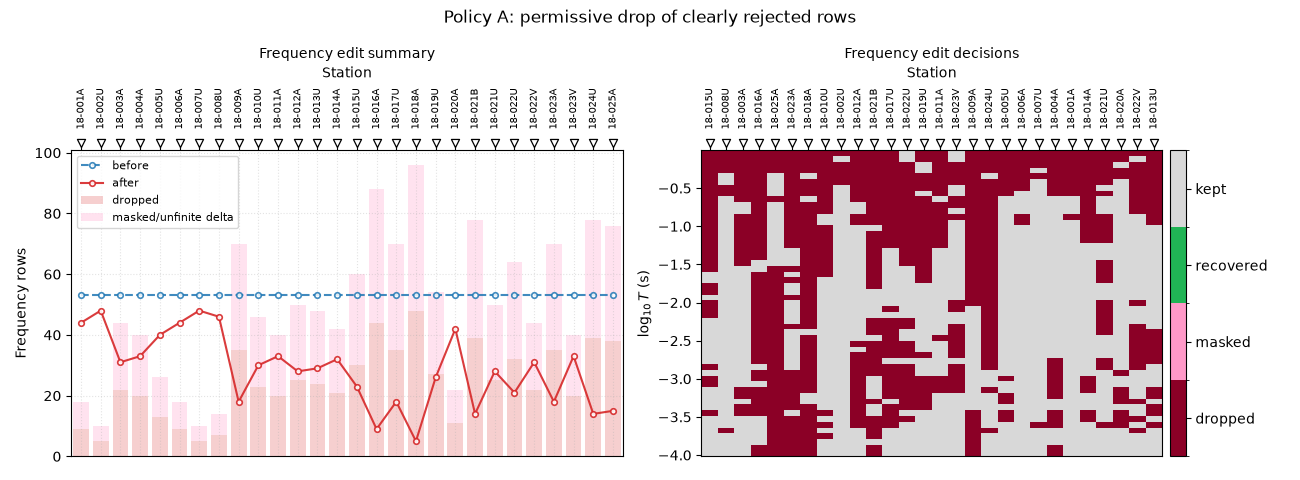
The permissive policy drops only rows below ci_lo. It is appropriate when downstream corrections can tolerate marginal rows, or when preserving frequency coverage is more important than removing every weak sample.

permissive = edit_frequencies_by_confidence(
    raw_for_permissive,
    before_sites=baseline,
    mode="drop",
    method="composite",
    threshold=permissive_threshold,
    also="z",
    recursive=False,
)

print(permissive.summary())
print("Permissive decisions:")
print(permissive.decisions["action"].value_counts(dropna=False).to_string())
print("Permissive station report, first rows:")
print(permissive.report.head(8).to_string(index=False))

fig, axs = plt.subplots(1, 2, figsize=(13.0, 4.8))
plot_frequency_edit_summary(
    baseline,
    permissive.sites,
    method="composite",
    ci_hi=ci_hi,
    ci_lo=ci_lo,
    ax=axs[0],
)
plot_frequency_edit_decisions(
    baseline,
    permissive.sites,
    method="composite",
    ci_hi=ci_hi,
    ci_lo=ci_lo,
    ax=axs[1],
)
fig.suptitle(
    "Policy A: permissive drop of clearly rejected rows", fontsize=12
)
fig.tight_layout()

APIResult(name='frequency_edit', kind='emtools.frequency.edit', keys=tuple(len=12, sample=['sites', 'report', 'decisions', ...]))
Permissive decisions:
action
kept       801
dropped    683
Permissive station report, first rows:
station  n_freq_before  n_finite_before  frac_finite_before  n_freq_after  n_finite_after  frac_finite_after  confidence_median_before  safe_fraction_before  recoverable_fraction_before  reject_fraction_before  confidence_median_after  safe_fraction_after  recoverable_fraction_after  reject_fraction_after  n_dropped  n_masked_or_unfinite  confidence_delta
18-001A             53               53                 1.0            44              44                1.0                  0.702527                   0.0                     0.981132                0.018868                 0.720398                  0.0                         1.0                    0.0          9                     9          0.017871
18-002U             53               53                 1.0            48              48                1.0                  0.725523                   0.0                     1.000000                0.000000                 0.719574                  0.0                         1.0                    0.0          5                     5         -0.005948
18-003A             53               53                 1.0            31              31                1.0                  0.668071                   0.0                     0.962264                0.037736                 0.701782                  0.0                         1.0                    0.0         22                    22          0.033711
18-004A             53               53                 1.0            33              33                1.0                  0.685382                   0.0                     0.924528                0.075472                 0.745365                  0.0                         1.0                    0.0         20                    20          0.059983
18-005U             53               53                 1.0            40              40                1.0                  0.680343                   0.0                     1.000000                0.000000                 0.737635                  0.0                         1.0                    0.0         13                    13          0.057292
18-006A             53               53                 1.0            44              44                1.0                  0.764254                   0.0                     0.886792                0.113208                 0.770054                  0.0                         1.0                    0.0          9                     9          0.005800
18-007U             53               53                 1.0            48              48                1.0                  0.780866                   0.0                     1.000000                0.000000                 0.779216                  0.0                         1.0                    0.0          5                     5         -0.001649
18-008U             53               53                 1.0            46              46                1.0                  0.718712                   0.0                     1.000000                0.000000                 0.703856                  0.0                         1.0                    0.0          7                     7         -0.014856

4. Policy B: conservative drop

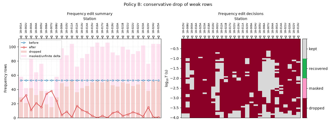
The conservative policy uses a higher threshold. It is attractive before static-shift or inversion when you want a cleaner input even if the frequency grid becomes thinner.

conservative = edit_frequencies_by_confidence(
    raw_for_conservative,
    before_sites=baseline,
    mode="drop",
    method="composite",
    threshold=conservative_threshold,
    ci_hi=ci_hi,
    ci_lo=ci_lo,
    also="z",
    recursive=False,
)

print(conservative.summary())
print("Conservative decisions:")
print(conservative.decisions["action"].value_counts(dropna=False).to_string())

fig, axs = plt.subplots(1, 2, figsize=(13.0, 4.8))
plot_frequency_edit_summary(
    baseline,
    conservative.sites,
    method="composite",
    ci_hi=ci_hi,
    ci_lo=ci_lo,
    ax=axs[0],
)
plot_frequency_edit_decisions(
    baseline,
    conservative.sites,
    method="composite",
    ci_hi=ci_hi,
    ci_lo=ci_lo,
    ax=axs[1],
)
fig.suptitle("Policy B: conservative drop of weak rows", fontsize=12)
fig.tight_layout()

APIResult(name='frequency_edit', kind='emtools.frequency.edit', keys=tuple(len=12, sample=['sites', 'report', 'decisions', ...]))
Conservative decisions:
action
dropped    1172
kept        312

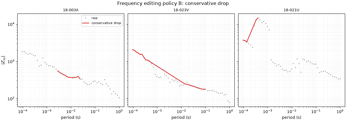
5. Compare the effect on sounding curves

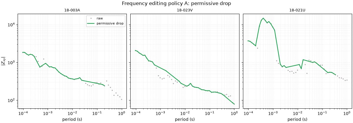
The plotted curves make the difference concrete. The permissive version keeps more samples; the conservative version removes more weak rows.

def impedance_magnitude_curves(sites, component="xy"):
    ij = {"xx": (0, 0), "xy": (0, 1), "yx": (1, 0), "yy": (1, 1)}[component]
    out = {}
    for i, ed in enumerate(_iter_items(sites)):
        _Z, z, fr = _get_z_block(ed)
        if z is None or fr is None:
            continue
        period = 1.0 / np.asarray(fr, dtype=float)
        out[_name(ed, i)] = (period, np.abs(np.asarray(z)[:, ij[0], ij[1]]))
    return out


def plot_impedance_compare(before, after, selected, *, label, color, title):
    common_selected = [station for station in selected if station in after]
    if len(common_selected) == 0:
        raise RuntimeError(
            "No selected stations are available after frequency editing."
        )
    fig, axes = plt.subplots(
        1,
        len(common_selected),
        figsize=(4.0 * len(common_selected), 4.2),
        sharey=True,
        constrained_layout=True,
    )
    if len(common_selected) == 1:
        axes = [axes]
    for ax, station in zip(axes, common_selected):
        pb, vb = before[station]
        pa, va = after[station]
        ax.loglog(pb, vb, ".", ms=3, color="#a8a29e", label="raw")
        ax.loglog(pa, va, "-", lw=1.7, color=color, label=label)
        ax.set_title(station, fontsize=9)
        ax.set_xlabel("period (s)")
        ax.grid(True, which="both", ls=":", lw=0.4, alpha=0.6)
    axes[0].set_ylabel(r"$|Z_{xy}|$")
    axes[0].legend(fontsize=8, framealpha=0.85)
    fig.suptitle(title, fontsize=12)
    return fig


raw_curves = impedance_magnitude_curves(baseline, component="xy")
permissive_curves = impedance_magnitude_curves(
    permissive.sites, component="xy"
)
conservative_curves = impedance_magnitude_curves(
    conservative.sites, component="xy"
)
common_stations = [
    station
    for station in raw_curves
    if station in permissive_curves and station in conservative_curves
]
if len(common_stations) < 3:
    raise RuntimeError(
        "Need at least three stations shared by both editing policies."
    )
pick = [
    common_stations[2],
    common_stations[len(common_stations) // 2],
    common_stations[-4],
]

plot_impedance_compare(
    raw_curves,
    permissive_curves,
    pick,
    label="permissive drop",
    color="#16a34a",
    title="Frequency editing policy A: permissive drop",
)

plot_impedance_compare(
    raw_curves,
    conservative_curves,
    pick,
    label="conservative drop",
    color="#dc2626",
    title="Frequency editing policy B: conservative drop",
)

• 
• 

<Figure size 1200x420 with 3 Axes>

6. Decision guide

Use the permissive policy when the rejected rows are rare and maintaining frequency coverage matters. Use the conservative policy when the confidence problem is broad, frequency-localized, or tied to instrument/source artefacts. In both cases, keep the decision table with your processing record; it is the audit trail for why a frequency survived or was removed.