Interpretation#

Turning a resistivity model into subsurface answers with pycsamt.interp — lithology, hydrogeology, petrophysics, calibration against boreholes, time-lapse monitoring, and uncertainty. One example per theme, each ending in a publication-style figure and a short reading guide.

The section works from a single synthetic 2-D resistivity section (a classic overburden / sand-aquifer / clay / resistive-basement sequence with lateral structure), so every deliverable is traceable to the same model:

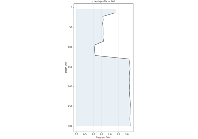
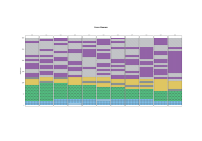
Resistivity model — the ResistivityModel container and 1-D depth profiles;
Lithology — rock-type classification and stratigraphic / fence logs;
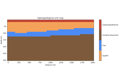
Hydro interpretation — qualitative aquifer-zone mapping;
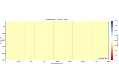
Hydro-geophysics — quantitative porosity, saturation, hydraulic conductivity, water table and transmissivity;
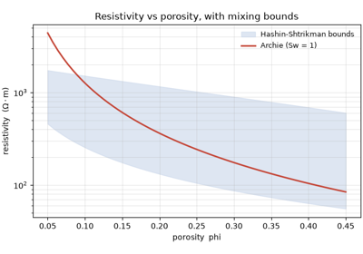
Petrophysics — Archie / Waxman-Smits rock-physics and cross-plots;
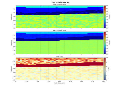
Calibration — tying the model to borehole ground truth;
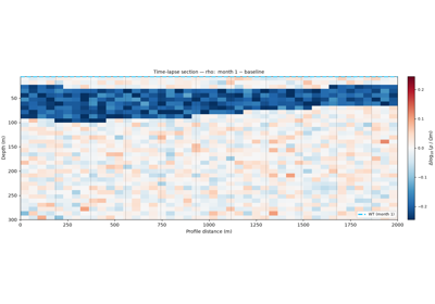
Time-lapse — differencing repeat surveys for monitoring;
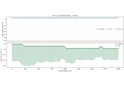
Uncertainty — Monte-Carlo propagation of petrophysical priors.

Every figure is produced by the plotting classes in pycsamt.interp.plot and regenerated on each documentation build. See the interpretation API reference for the full listing.