
Note
Go to the end to download the full example code.
Full inversion case study: from field data to interpretation package#
This case study brings together the pieces used throughout the inversion gallery. It is written as a guided workflow for a user who has collected EDI data, prepared inversion files, run one or more solvers, and now needs to make a defensible interpretation.
The repository contains three useful kinds of example material:
EDI survey data in
data/AMT/WILLY_DATA;Occam2D input/result artefacts in
data/oc2_input_filesanddata/occam2D;ModEM result artefacts in
data/modem/willy_27freq_watex_line02_sample.
The objective is not to force Occam and ModEM to agree perfectly. They are different inversion approaches with different parameterizations. The objective is to teach a robust interpretation habit:
audit the available data and inversion artefacts;
inspect convergence before interpreting the model;
compare observed and predicted responses;
compare solver/scenario evidence;
write clear caveats for the final report.
The script is intentionally verbose. It is a teaching example, so comments explain why each diagnostic is useful, not only how to compute it.
1. Imports and paths#
import json
import os
import sys
from pathlib import Path

# sphinx-gallery executes examples without __file__ (the gallery
# runner sets the working directory to this example's folder).
try:
    EXAMPLE_DIR = Path(__file__).resolve().parent
except NameError:
    EXAMPLE_DIR = Path.cwd()

import matplotlib.pyplot as plt
import numpy as np
import pandas as pd


def repo_root():
    root = os.environ.get("PYCSAMT_DOCS_REPO_ROOT")
    return Path(root) if root else EXAMPLE_DIR.parents[2]


ROOT = repo_root()
if str(ROOT) not in sys.path:
    sys.path.insert(0, str(ROOT))

from pycsamt.models.modem import InversionResult
from pycsamt.models.occam2d import OccamLog

data_root = ROOT / "data"
edi_line = data_root / "AMT" / "WILLY_DATA" / "L18PLT"
occam_input = data_root / "oc2_input_files"
occam_result = data_root / "occam2D"
modem_result = data_root / "modem" / "willy_27freq_watex_line02_sample"

case_root = EXAMPLE_DIR / "workspaces" / "case_study_l18"
figure_dir = case_root / "figures"
table_dir = case_root / "tables"
report_dir = case_root / "report"

for path in (figure_dir, table_dir, report_dir):
    path.mkdir(parents=True, exist_ok=True)
2. Inventory the available project evidence#
A good interpretation starts with an inventory. This avoids a surprisingly common mistake: interpreting a model without knowing which input files, response files, or logs were actually present.
def inventory_folder(folder, label):
    folder = Path(folder)
    rows = []
    if not folder.exists():
        return pd.DataFrame(
            [
                {
                    "group": label,
                    "file": "",
                    "suffix": "",
                    "size_bytes": 0,
                    "exists": False,
                }
            ]
        )
    for path in sorted(folder.rglob("*")):
        if path.is_file():
            rows.append(
                {
                    "group": label,
                    "file": str(path.relative_to(folder)),
                    "suffix": path.suffix or path.name,
                    "size_bytes": path.stat().st_size,
                    "exists": True,
                }
            )
    return pd.DataFrame(rows)


inventory = pd.concat(
    [
        inventory_folder(edi_line, "EDI line"),
        inventory_folder(occam_input, "Occam input"),
        inventory_folder(occam_result, "Occam result"),
        inventory_folder(modem_result, "ModEM result"),
    ],
    ignore_index=True,
)
inventory_file = table_dir / "case_study_file_inventory.csv"
inventory.to_csv(inventory_file, index=False)

print("Inventory summary:")
print(
    inventory.groupby("group")
    .agg(
        n_files=("file", "count"),
        total_mb=("size_bytes", lambda s: s.sum() / 1e6),
    )
    .round(3)
    .to_string()
)
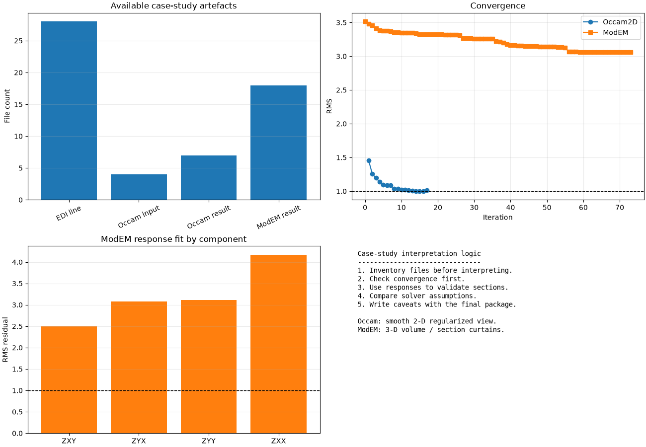
Inventory summary:
              n_files  total_mb
group
EDI line           28     0.627
ModEM result       18    43.388
Occam input         1     0.000
Occam result        7     0.439
3. Read convergence logs from Occam and ModEM#
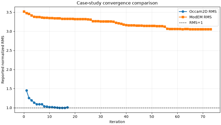
Convergence is the first interpretation gate. If a run did not stabilize, its model section may still be useful diagnostically, but it should not be presented as a final geological result without caveats.
occam_log_file = occam_result / "LogFile.logfile"
occam_summary = {
    "available": occam_log_file.exists(),
    "n_iter": 0,
    "final_rms": np.nan,
    "best_iteration": 0,
    "best_rms": np.nan,
    "converged": False,
}

if occam_log_file.exists():
    occam_log = OccamLog.read(occam_log_file)
    finite_rms = occam_log.rms[np.isfinite(occam_log.rms)]
    occam_summary.update(
        {
            "n_iter": int(occam_log.n_iter),
            "final_rms": float(occam_log.rms[-1])
            if occam_log.rms.size
            else np.nan,
            "best_iteration": int(occam_log.best_iteration),
            "best_rms": float(np.nanmin(finite_rms))
            if finite_rms.size
            else np.nan,
            "converged": bool(occam_log.converged),
        }
    )
else:
    occam_log = None

modem_summary = {
    "available": modem_result.exists(),
    "n_iter": 0,
    "final_rms": np.nan,
    "best_iteration": 0,
    "best_rms": np.nan,
    "mode": "",
}

if modem_result.exists():
    modem = InversionResult(
        modem_result,
        load_control=False,
        load_covariance=False,
        load_models=False,
    )
    modem_summary.update(
        {
            "n_iter": int(modem.n_iter),
            "final_rms": float(modem.final_rms),
            "best_iteration": int(modem.log.best_iter) if modem.log else 0,
            "best_rms": float(modem.best_rms),
            "mode": modem.mode,
        }
    )
else:
    modem = None

convergence_summary = pd.DataFrame(
    [
        {"solver": "Occam2D", **occam_summary},
        {"solver": "ModEM", **modem_summary},
    ]
)
convergence_file = table_dir / "case_study_convergence_summary.csv"
convergence_summary.to_csv(convergence_file, index=False)

print("Convergence summary:")
print(convergence_summary.to_string(index=False))
Convergence summary:
 solver  available  n_iter  final_rms  best_iteration  best_rms converged mode
Occam2D       True      17   1.013065              16  0.997701      True  NaN
  ModEM       True      74   3.057151              73  3.057151       NaN   3d
4. Plot convergence comparison#
Occam and ModEM RMS values are not always directly interchangeable because they may use different data selections, error floors, and objective functions. Still, plotting them together is useful as a diagnostic: it shows whether each run is still improving or has flattened.
fig_conv, ax_conv = plt.subplots(figsize=(8.5, 4.8), constrained_layout=True)

if occam_log is not None and occam_log.rms.size:
    ax_conv.plot(
        occam_log.iterations,
        occam_log.rms,
        "o-",
        label="Occam2D RMS",
        linewidth=2,
    )

if modem is not None and modem.rms_history.size:
    ax_conv.plot(
        modem.iteration_numbers,
        modem.rms_history,
        "s-",
        label="ModEM RMS",
        linewidth=2,
    )

ax_conv.axhline(
    1.0, color="black", linestyle="--", linewidth=1.0, label="RMS=1"
)
ax_conv.set_xlabel("Iteration")
ax_conv.set_ylabel("Reported normalized RMS")
ax_conv.set_title("Case-study convergence comparison")
ax_conv.grid(alpha=0.25)
ax_conv.legend()
convergence_plot = figure_dir / "case_study_convergence_comparison.png"
fig_conv.savefig(convergence_plot, dpi=120)
plt.show()
5. Summarize response evidence#
For ModEM we can compare observed and predicted response rows from the sample.
For Occam, the available .dat and .resp files are recorded in the
inventory and can be plotted by Occam-specific tools in a more specialized
example. Here we compute a compact ModEM response residual summary.
def modem_data_frame(data, source):
    rows = []
    if data is None:
        return pd.DataFrame(rows)
    for block in data.blocks:
        for row in block["rows"]:
            period, site_idx, x_m, y_m, z_m, comp, real, imag, error = row
            rows.append(
                {
                    "source": source,
                    "station": data.site_names[int(site_idx)],
                    "period_s": float(period),
                    "component": str(comp).upper(),
                    "real": float(real),
                    "imag": float(imag),
                    "error": float(error),
                    "x_m": float(x_m),
                    "y_m": float(y_m),
                    "z_m": float(z_m),
                }
            )
    return pd.DataFrame(rows)


response_summary = pd.DataFrame()
if (
    modem is not None
    and modem.data_obs is not None
    and modem.data_pred is not None
):
    obs = modem_data_frame(modem.data_obs, "observed")
    pred = modem_data_frame(modem.data_pred, "predicted")
    matched = obs.merge(
        pred,
        on=["station", "period_s", "component"],
        suffixes=("_obs", "_pred"),
    )
    matched = matched[matched["error_obs"].between(0.0, 1.0e10)].copy()
    matched["real_residual"] = (
        matched["real_obs"] - matched["real_pred"]
    ) / matched["error_obs"]
    matched["imag_residual"] = (
        matched["imag_obs"] - matched["imag_pred"]
    ) / matched["error_obs"]
    matched["combined_residual"] = np.sqrt(
        0.5 * (matched["real_residual"] ** 2 + matched["imag_residual"] ** 2)
    )
    response_summary = (
        matched.groupby("component")
        .agg(
            n_rows=("combined_residual", "size"),
            rms_residual=(
                "combined_residual",
                lambda s: float(np.sqrt(np.nanmean(np.asarray(s) ** 2))),
            ),
            median_abs_residual=(
                "combined_residual",
                lambda s: float(np.nanmedian(np.abs(s))),
            ),
        )
        .reset_index()
        .sort_values("rms_residual")
    )
    matched.to_csv(
        table_dir / "case_study_modem_matched_response_rows.csv", index=False
    )

response_file = table_dir / "case_study_response_component_summary.csv"
response_summary.to_csv(response_file, index=False)

print("Response component summary:")
print(
    response_summary.to_string(index=False)
    if not response_summary.empty
    else "No matched ModEM responses."
)
Response component summary:
component  n_rows  rms_residual  median_abs_residual
      ZXY     373      2.492944             2.271678
      ZYX     373      3.083097             2.207043
      ZYY     373      3.118287             1.524132
      ZXX     373      4.164972             2.194044
6. Compare solver evidence as a decision table#
This table is the heart of the case study. It does not pretend that Occam and ModEM answer the exact same numerical question. Instead, it records what each solver contributes to the interpretation.
decision_rows = [
    {
        "evidence": "EDI data availability",
        "Occam2D": "Uses OccamDataFile prepared from survey data",
        "ModEM": "Uses ModEM .dat input and predicted responses",
        "interpretation_value": "Confirms both workflows are grounded in field responses.",
    },
    {
        "evidence": "Convergence",
        "Occam2D": (
            f"{occam_summary['n_iter']} iterations, final RMS "
            f"{occam_summary['final_rms']:.3g}"
            if occam_summary["available"]
            else "No log available"
        ),
        "ModEM": (
            f"{modem_summary['n_iter']} records, final RMS "
            f"{modem_summary['final_rms']:.3g}"
            if modem_summary["available"]
            else "No log available"
        ),
        "interpretation_value": "Shows whether each inversion is stable enough to interpret.",
    },
    {
        "evidence": "Model geometry",
        "Occam2D": "Native 2-D smooth section",
        "ModEM": f"{modem_summary.get('mode', 'unknown')} volume; sections are extracted curtains",
        "interpretation_value": "Explains why sections may differ even with similar data.",
    },
    {
        "evidence": "Response fit",
        "Occam2D": "RESP17.resp available for Occam response checks",
        "ModEM": (
            "Observed/predicted rows matched by station, period, component"
            if not response_summary.empty
            else "No matched response table"
        ),
        "interpretation_value": "Identifies stations/periods that still control misfit.",
    },
    {
        "evidence": "Report caveat",
        "Occam2D": "Smooth model may suppress sharp/local 3-D features",
        "ModEM": "3-D model may add structure that requires response support",
        "interpretation_value": "Prevents overclaiming solver-specific artefacts.",
    },
]

decision_table = pd.DataFrame(decision_rows)
decision_file = table_dir / "case_study_solver_evidence_table.csv"
decision_table.to_csv(decision_file, index=False)
print("Decision table:")
print(decision_table.to_string(index=False))
Decision table:
             evidence                                            Occam2D                                                         ModEM                                        interpretation_value
EDI data availability       Uses OccamDataFile prepared from survey data                 Uses ModEM .dat input and predicted responses    Confirms both workflows are grounded in field responses.
          Convergence                      17 iterations, final RMS 1.01                                    74 records, final RMS 3.06 Shows whether each inversion is stable enough to interpret.
       Model geometry                          Native 2-D smooth section                    3d volume; sections are extracted curtains    Explains why sections may differ even with similar data.
         Response fit    RESP17.resp available for Occam response checks Observed/predicted rows matched by station, period, component      Identifies stations/periods that still control misfit.
        Report caveat Smooth model may suppress sharp/local 3-D features    3-D model may add structure that requires response support            Prevents overclaiming solver-specific artefacts.
7. Build a case-study dashboard#
The dashboard gives a project manager or report reviewer a quick overview: what files exist, how the runs converged, and what response evidence is available. It is not a substitute for detailed response and model plots.
fig, axes = plt.subplots(2, 2, figsize=(13.0, 9.0), constrained_layout=True)
ax_inv, ax_rms, ax_resp, ax_notes = axes.ravel()

inv_summary = (
    inventory.groupby("group")["file"]
    .count()
    .reindex(["EDI line", "Occam input", "Occam result", "ModEM result"])
)
ax_inv.bar(inv_summary.index, inv_summary.values, color="tab:blue")
ax_inv.set_title("Available case-study artefacts")
ax_inv.set_ylabel("File count")
ax_inv.tick_params(axis="x", rotation=25)
ax_inv.grid(axis="y", alpha=0.25)

if occam_log is not None and occam_log.rms.size:
    ax_rms.plot(occam_log.iterations, occam_log.rms, "o-", label="Occam2D")
if modem is not None and modem.rms_history.size:
    ax_rms.plot(
        modem.iteration_numbers, modem.rms_history, "s-", label="ModEM"
    )
ax_rms.axhline(1.0, color="black", linestyle="--", linewidth=1.0)
ax_rms.set_title("Convergence")
ax_rms.set_xlabel("Iteration")
ax_rms.set_ylabel("RMS")
ax_rms.legend()
ax_rms.grid(alpha=0.25)

if not response_summary.empty:
    ax_resp.bar(
        response_summary["component"],
        response_summary["rms_residual"],
        color="tab:orange",
    )
    ax_resp.axhline(1.0, color="black", linestyle="--", linewidth=1.0)
    ax_resp.set_ylabel("RMS residual")
else:
    ax_resp.text(0.5, 0.5, "No response summary", ha="center", va="center")
ax_resp.set_title("ModEM response fit by component")
ax_resp.grid(axis="y", alpha=0.25)

note_lines = [
    "Case-study interpretation logic",
    "-------------------------------",
    "1. Inventory files before interpreting.",
    "2. Check convergence first.",
    "3. Use responses to validate sections.",
    "4. Compare solver assumptions.",
    "5. Write caveats with the final package.",
    "",
    "Occam: smooth 2-D regularized view.",
    "ModEM: 3-D volume / section curtains.",
]
ax_notes.axis("off")
ax_notes.text(
    0.02,
    0.98,
    "\n".join(note_lines),
    va="top",
    family="monospace",
    fontsize=10,
)

dashboard_file = figure_dir / "case_study_interpretation_dashboard.png"
fig.savefig(dashboard_file, dpi=120)
plt.show()
8. Write a guided case-study memo#
This memo is the narrative bridge from computation to report. It captures what the user should say in a real project handoff.
memo = [
    "# Inversion case-study memo",
    "",
    "## Study objective",
    "",
    "Use EDI data, Occam2D artefacts, and ModEM result samples to demonstrate "
    "a defensible interpretation workflow from field data to final reporting.",
    "",
    "## Evidence used",
    "",
    f"- EDI line folder: `{edi_line}`",
    f"- Occam input folder: `{occam_input}`",
    f"- Occam result folder: `{occam_result}`",
    f"- ModEM result folder: `{modem_result}`",
    "",
    "## Main interpretation checks",
    "",
    "1. File inventory was written before model interpretation.",
    "2. Occam and ModEM convergence histories were summarized.",
    "3. ModEM observed/predicted responses were matched where available.",
    "4. Solver assumptions were compared in a decision table.",
    "5. Caveats were stated explicitly.",
    "",
    "## Solver-specific guidance",
    "",
    "- Occam2D is useful for a smooth, conservative section.  It can be easier "
    "to explain, but it may smear compact 3-D structures.",
    "- ModEM can represent 3-D structure, but extracted 2-D sections should be "
    "checked against response residuals before being interpreted as geology.",
    "",
    "## Recommended next checks",
    "",
    "- Plot station-level response residuals for the worst-fitting components.",
    "- Compare Occam response files against ModEM predicted responses where the "
    "same stations/frequencies are available.",
    "- Review whether the same conductive/resistive zones appear in both smooth "
    "2-D and 3-D-derived sections.",
    "- Carry uncertainty/caveats into the final interpretation package.",
]
memo_file = report_dir / "case_study_interpretation_memo.md"
memo_file.write_text("\n".join(memo) + "\n", encoding="utf-8")

case_manifest = {
    "inventory": str(inventory_file),
    "convergence_summary": str(convergence_file),
    "convergence_plot": str(convergence_plot),
    "response_component_summary": str(response_file),
    "solver_evidence_table": str(decision_file),
    "dashboard": str(dashboard_file),
    "memo": str(memo_file),
}
manifest_file = report_dir / "case_study_outputs.json"
manifest_file.write_text(json.dumps(case_manifest, indent=2), encoding="utf-8")

print(f"Inventory: {inventory_file}")
print(f"Convergence summary: {convergence_file}")
print(f"Convergence plot: {convergence_plot}")
print(f"Response summary: {response_file}")
print(f"Solver evidence table: {decision_file}")
print(f"Dashboard: {dashboard_file}")
print(f"Memo: {memo_file}")
print(f"Output manifest: {manifest_file}")
Inventory: /opt/build/repo/docs/examples/inversion/workspaces/case_study_l18/tables/case_study_file_inventory.csv
Convergence summary: /opt/build/repo/docs/examples/inversion/workspaces/case_study_l18/tables/case_study_convergence_summary.csv
Convergence plot: /opt/build/repo/docs/examples/inversion/workspaces/case_study_l18/figures/case_study_convergence_comparison.png
Response summary: /opt/build/repo/docs/examples/inversion/workspaces/case_study_l18/tables/case_study_response_component_summary.csv
Solver evidence table: /opt/build/repo/docs/examples/inversion/workspaces/case_study_l18/tables/case_study_solver_evidence_table.csv
Dashboard: /opt/build/repo/docs/examples/inversion/workspaces/case_study_l18/figures/case_study_interpretation_dashboard.png
Memo: /opt/build/repo/docs/examples/inversion/workspaces/case_study_l18/report/case_study_interpretation_memo.md
Output manifest: /opt/build/repo/docs/examples/inversion/workspaces/case_study_l18/report/case_study_outputs.json
9. How to use this case study with your own data#
Replace the four source folders at the top of the script:
edi_linewith your corrected EDI folder;occam_inputwith your Occam input folder;occam_resultwith your completed Occam run;modem_resultwith your completed ModEM run.
Then rerun the same audit:
Do the files exist?
Did convergence stabilize?
Which stations/components still have high residuals?
Are the same geological features stable across solvers/scenarios?
What caveats must appear in the report?
This is the mindset that makes inversion results reproducible and defensible.
Total running time of the script: (0 minutes 0.831 seconds)