
Note
Go to the end to download the full example code.
Compare observed vs predicted responses#
An inversion section is only convincing if the predicted data reproduce the observations. After plotting a model, the next diagnostic is therefore a response comparison:
observed apparent resistivity and phase curves;
predicted/modelled curves from the inversion;
normalized residuals by station, component, and period.
This example uses the compact ModEM result sample in data/modem. It first
uses pyCSAMT’s built-in PlotResponse helper, then builds explicit
tables and residual plots so the user can decide which stations or periods are
controlling the remaining misfit.
The important habit is this: do not accept a pretty model until you know where it does not fit the data.
1. Imports and paths#
import os
import sys
from pathlib import Path

# sphinx-gallery executes examples without __file__ (the gallery
# runner sets the working directory to this example's folder).
try:
    EXAMPLE_DIR = Path(__file__).resolve().parent
except NameError:
    EXAMPLE_DIR = Path.cwd()

import matplotlib.pyplot as plt
import numpy as np
import pandas as pd


def repo_root():
    root = os.environ.get("PYCSAMT_DOCS_REPO_ROOT")
    return Path(root) if root else EXAMPLE_DIR.parents[2]


ROOT = repo_root()
if str(ROOT) not in sys.path:
    sys.path.insert(0, str(ROOT))

from pycsamt.models.modem import InversionResult, PlotPseudo, PlotResponse

sample_dir = ROOT / "data" / "modem" / "willy_27freq_watex_line02_sample"
figure_dir = EXAMPLE_DIR / "workspaces" / "modem_result_figures"
table_dir = EXAMPLE_DIR / "workspaces" / "modem_result_tables"

for path in (figure_dir, table_dir):
    path.mkdir(parents=True, exist_ok=True)

if not sample_dir.exists():
    raise RuntimeError(f"Missing ModEM sample directory: {sample_dir}")
2. Load the result and check what is available#
InversionResult chooses the observed data file and the latest numbered
predicted data file when it scans the folder. For this compact sample, the
latest copied response is Modular_NLCG_073.dat.
result = InversionResult(
    sample_dir,
    load_control=False,
    load_covariance=False,
    load_models=False,
)

if result.data_obs is None:
    raise RuntimeError("The ModEM sample did not provide observed data.")
if result.data_pred is None:
    raise RuntimeError("The ModEM sample did not provide predicted data.")

print(result)
print(f"Observed sites: {result.data_obs.n_sites}")
print(f"Observed periods: {result.data_obs.n_periods}")
print(f"Predicted sites: {result.data_pred.n_sites}")
print(f"Predicted periods: {result.data_pred.n_periods}")
print(f"Final RMS from log: {result.final_rms:.3f}")
InversionResult(mode='3d', n_iter=74, final_rms=3.0572, models=[])
Observed sites: 125
Observed periods: 27
Predicted sites: 125
Predicted periods: 27
Final RMS from log: 3.057
3. Convert ModEM data blocks to analysis tables#
ModEM data files store real and imaginary response values, one row per station/period/component. For response QA we convert the blocks into a tidy table. Rows with huge sentinel errors are excluded from residual statistics because ModEM uses those errors to mark masked or inactive data.
ERROR_SENTINEL = 1.0e10


def data_to_frame(data, source):
    rows = []
    for block in data.blocks:
        component_type = block["component_type"]
        for row in block["rows"]:
            period, site_idx, x_m, y_m, z_m, component, real, imag, error = row
            station = data.site_names[int(site_idx)]
            rows.append(
                {
                    "source": source,
                    "component_type": component_type,
                    "station": station,
                    "period_s": float(period),
                    "frequency_hz": 1.0 / float(period),
                    "x_m": float(x_m),
                    "y_m": float(y_m),
                    "z_m": float(z_m),
                    "component": str(component).upper(),
                    "real": float(real),
                    "imag": float(imag),
                    "error": float(error),
                }
            )
    return pd.DataFrame(rows)


observed = data_to_frame(result.data_obs, "observed")
predicted = data_to_frame(result.data_pred, "predicted")

print("Observed components:", sorted(observed["component"].unique()))
print("Predicted components:", sorted(predicted["component"].unique()))
Observed components: ['ZXX', 'ZXY', 'ZYX', 'ZYY']
Predicted components: ['ZXX', 'ZXY', 'ZYX', 'ZYY']
4. Match observed and predicted rows#
We match by station, period, and component. This is stricter than simply plotting the two files because it allows quantitative residual checks. The normalized residual uses the same idea as inversion RMS:
residual = (observed - predicted) / assigned_error
Real and imaginary parts are kept separately, then combined into station and component RMS summaries.
join_cols = ["station", "period_s", "component"]
matched = observed.merge(
    predicted,
    on=join_cols,
    suffixes=("_obs", "_pred"),
    how="inner",
)

matched = matched[matched["error_obs"].between(0.0, ERROR_SENTINEL)].copy()
matched["real_residual"] = (
    matched["real_obs"] - matched["real_pred"]
) / matched["error_obs"]
matched["imag_residual"] = (
    matched["imag_obs"] - matched["imag_pred"]
) / matched["error_obs"]
matched["combined_rms_residual"] = np.sqrt(
    0.5 * (matched["real_residual"] ** 2 + matched["imag_residual"] ** 2)
)

matched["z_abs_obs"] = np.hypot(matched["real_obs"], matched["imag_obs"])
matched["z_abs_pred"] = np.hypot(matched["real_pred"], matched["imag_pred"])
matched["z_abs_ratio_pred_obs"] = matched["z_abs_pred"] / matched["z_abs_obs"]

with np.errstate(divide="ignore", invalid="ignore"):
    matched["phase_obs_deg"] = np.degrees(
        np.arctan2(matched["imag_obs"], matched["real_obs"])
    )
    matched["phase_pred_deg"] = np.degrees(
        np.arctan2(matched["imag_pred"], matched["real_pred"])
    )
matched["phase_error_deg"] = (
    matched["phase_pred_deg"] - matched["phase_obs_deg"]
)

matched_file = table_dir / "modem_observed_predicted_matched_rows.csv"
matched.to_csv(matched_file, index=False)

print(f"Matched active rows: {len(matched)}")
print(f"Matched table: {matched_file}")
Matched active rows: 1492
Matched table: /opt/build/repo/docs/examples/inversion/workspaces/modem_result_tables/modem_observed_predicted_matched_rows.csv
5. Select stations to inspect#
A response figure with every station can become unreadable. A useful gallery strategy is to show a few representative stations:
one of the best-fitting stations;
one median station;
one of the worst-fitting stations.
def rms(values):
    values = np.asarray(values, dtype=float)
    values = values[np.isfinite(values)]
    if values.size == 0:
        return np.nan
    return float(np.sqrt(np.mean(values**2)))


station_summary = (
    matched.groupby("station")
    .agg(
        n_rows=("combined_rms_residual", "size"),
        rms_real=("real_residual", rms),
        rms_imag=("imag_residual", rms),
        rms_combined=("combined_rms_residual", rms),
        median_abs_phase_error_deg=(
            "phase_error_deg",
            lambda s: float(np.nanmedian(np.abs(s))),
        ),
    )
    .sort_values("rms_combined")
)

station_summary_file = table_dir / "modem_response_station_misfit_summary.csv"
station_summary.to_csv(station_summary_file)

ordered_stations = list(station_summary.index)
selected_stations = [
    ordered_stations[0],
    ordered_stations[len(ordered_stations) // 2],
    ordered_stations[-1],
]
selected_stations = list(dict.fromkeys(selected_stations))

print("Selected stations for response panels:", selected_stations)
print("Station summary:")
print(station_summary.head(5).to_string())
print(station_summary.tail(5).to_string())
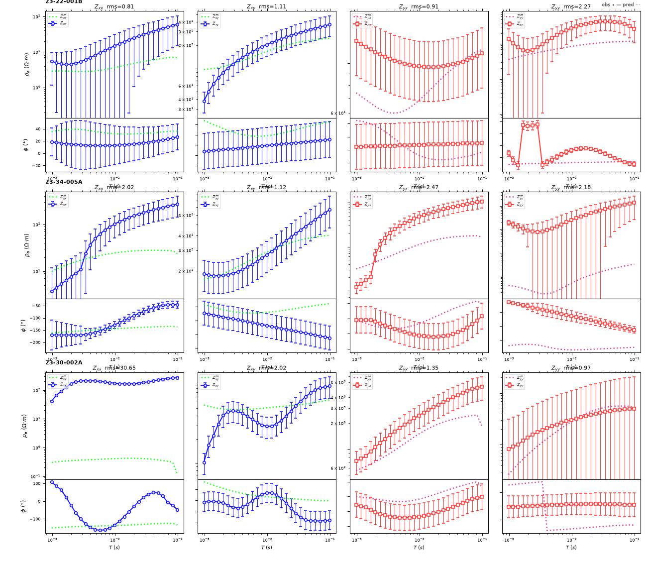
Selected stations for response panels: ['23-22-001B', '23-34-005A', '23-30-002A']
Station summary:
            n_rows  rms_real  rms_imag  rms_combined  median_abs_phase_error_deg
station
23-22-001B      12  1.114638  1.003948      1.060738                   10.191711
23-22-002V      12  1.591920  0.983354      1.323101                   22.096490
23-26-003U      12  1.616454  1.278778      1.457428                   13.643881
23-34-003A      12  1.772479  1.102619      1.476050                   16.922994
23-18-003A      12  1.793799  1.182920      1.519377                   21.867761
            n_rows   rms_real   rms_imag  rms_combined  median_abs_phase_error_deg
station
23-18-023A      12   5.566188   5.709550      5.638325                   84.645406
23-26-020A      12   3.830821   7.258715      5.803625                   95.183601
23-22-025A      12   3.897675   8.261180      6.459062                   74.317099
23-30-001U      12   6.782033  15.892253     12.218012                   33.658154
23-30-002A      12  15.682745  12.008553     13.966994                   52.354848
6. Plot observed and predicted response curves#
PlotResponse draws apparent-resistivity and phase curves for the selected
stations. Observed data are shown as error bars; predicted data are overlaid
as model curves. The subplot title reports component RMS where available.
fig_response = PlotResponse(
    result=result,
    stations=selected_stations,
    max_stations=len(selected_stations),
    period_min=None,
    period_max=None,
    figsize=(13.0, 3.8 * len(selected_stations)),
).plot()
response_file = figure_dir / "modem_observed_vs_predicted_response_panels.png"
fig_response.savefig(response_file, dpi=120)
plt.show()
7. Plot survey-scale pseudo-sections#
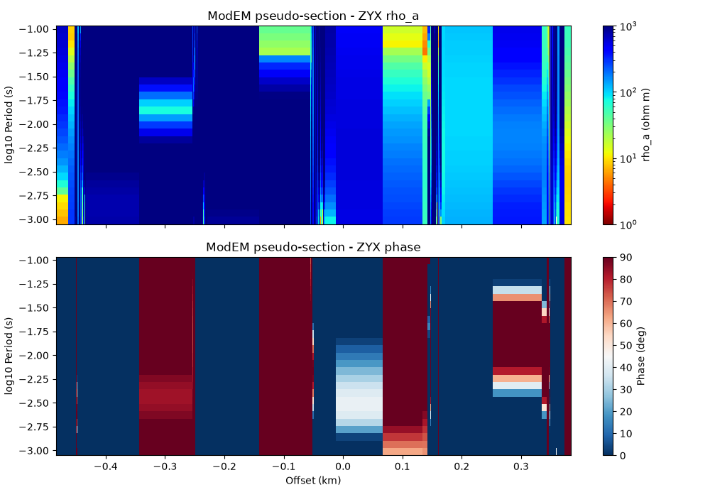
Curves are excellent for individual stations; pseudo-sections show whether the misfit is spatially organized. Here we draw observed pseudo-sections for the two off-diagonal components commonly used in MT/CSAMT interpretation. These plots are not residual maps yet; they provide the visual context for where periods and stations sit in the survey.
for component in ("ZXY", "ZYX"):
    fig_pseudo = PlotPseudo(result=result, component=component).plot()
    pseudo_file = figure_dir / f"modem_observed_pseudo_{component.lower()}.png"
    fig_pseudo.savefig(pseudo_file, dpi=120)
    plt.show()
    print(f"{component} pseudo-section: {pseudo_file}")
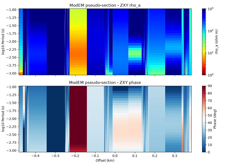
ZXY pseudo-section: /opt/build/repo/docs/examples/inversion/workspaces/modem_result_figures/modem_observed_pseudo_zxy.png
ZYX pseudo-section: /opt/build/repo/docs/examples/inversion/workspaces/modem_result_figures/modem_observed_pseudo_zyx.png
8. Build residual heatmaps#
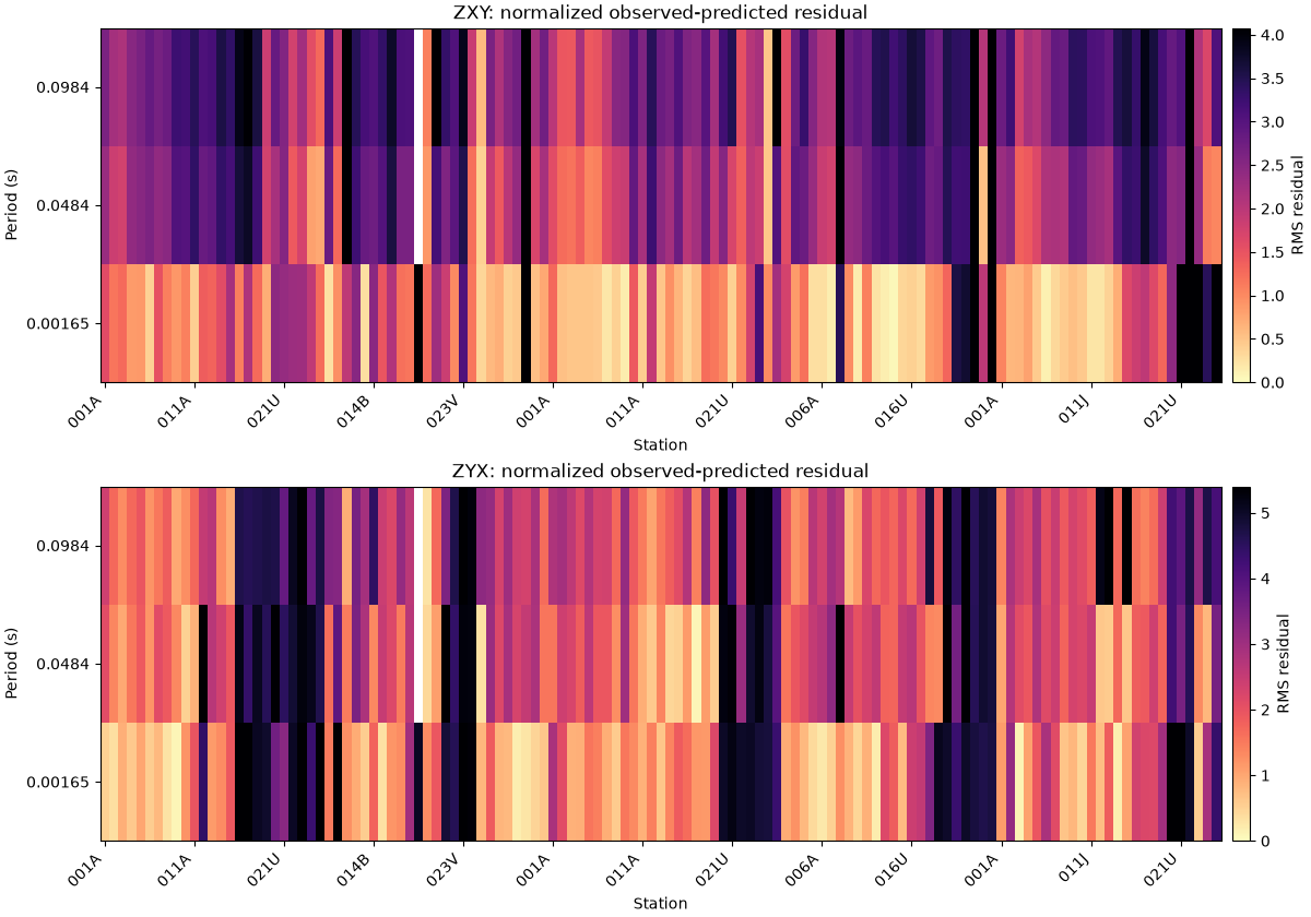
The heatmap below is often the most useful response QA figure. Values near one mean the prediction is within the assigned error on average. Coherent bands of high residual can indicate:
an error-floor problem at a period range;
a static-shift or near-surface effect not fully corrected;
a station with poor data quality;
a 3-D structure not captured by the selected model parametrization.
components_to_plot = ["ZXY", "ZYX"]
fig_heat, axes = plt.subplots(
    len(components_to_plot),
    1,
    figsize=(12.0, 4.2 * len(components_to_plot)),
    constrained_layout=True,
)
if len(components_to_plot) == 1:
    axes = [axes]

for ax, component in zip(axes, components_to_plot):
    subset = matched[matched["component"] == component].copy()
    pivot = subset.pivot_table(
        index="period_s",
        columns="station",
        values="combined_rms_residual",
        aggfunc="mean",
    )
    pivot = pivot.sort_index(ascending=False)
    pivot = pivot.reindex(columns=result.data_obs.site_names)

    im = ax.imshow(
        pivot.to_numpy(),
        aspect="auto",
        interpolation="nearest",
        vmin=0.0,
        vmax=max(4.0, float(np.nanpercentile(pivot.to_numpy(), 95))),
        cmap="magma_r",
    )
    ax.set_title(f"{component}: normalized observed-predicted residual")
    ax.set_ylabel("Period (s)")
    ax.set_xlabel("Station")

    y_positions = np.arange(len(pivot.index))
    y_step = max(1, len(y_positions) // 8)
    ax.set_yticks(y_positions[::y_step])
    ax.set_yticklabels([f"{p:.3g}" for p in pivot.index[::y_step]])

    x_positions = np.arange(len(pivot.columns))
    x_step = max(1, len(x_positions) // 12)
    ax.set_xticks(x_positions[::x_step])
    ax.set_xticklabels(
        [str(s).split("-")[-1] for s in pivot.columns[::x_step]],
        rotation=45,
        ha="right",
    )
    cbar = fig_heat.colorbar(im, ax=ax, pad=0.01)
    cbar.set_label("RMS residual")

heatmap_file = figure_dir / "modem_response_residual_heatmaps.png"
fig_heat.savefig(heatmap_file, dpi=120)
plt.show()
9. Summarize component-level fit#
A compact table is helpful when comparing multiple inversion attempts. If a new inversion lowers section roughness but worsens response RMS, this table makes the trade-off visible.
component_summary = (
    matched.groupby("component")
    .agg(
        n_rows=("combined_rms_residual", "size"),
        rms_real=("real_residual", rms),
        rms_imag=("imag_residual", rms),
        rms_combined=("combined_rms_residual", rms),
        median_abs_phase_error_deg=(
            "phase_error_deg",
            lambda s: float(np.nanmedian(np.abs(s))),
        ),
        median_pred_obs_amplitude_ratio=("z_abs_ratio_pred_obs", "median"),
    )
    .sort_values("rms_combined")
)
component_summary_file = (
    table_dir / "modem_response_component_misfit_summary.csv"
)
component_summary.to_csv(component_summary_file)

fig_bar, ax_bar = plt.subplots(figsize=(8.5, 4.6), constrained_layout=True)
component_summary["rms_combined"].plot.bar(ax=ax_bar, color="tab:blue")
ax_bar.axhline(1.0, color="black", linestyle="--", linewidth=1.0)
ax_bar.axhline(2.0, color="tab:orange", linestyle=":", linewidth=1.0)
ax_bar.set_ylabel("Combined normalized RMS residual")
ax_bar.set_xlabel("Component")
ax_bar.set_title("Component-level observed vs predicted fit")
ax_bar.grid(axis="y", alpha=0.25)
bar_file = figure_dir / "modem_response_component_rms_summary.png"
fig_bar.savefig(bar_file, dpi=120)
plt.show()

print("Component summary:")
print(component_summary.to_string())
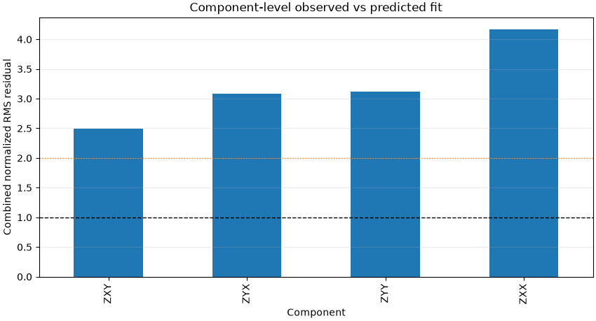
Component summary:
           n_rows  rms_real  rms_imag  rms_combined  median_abs_phase_error_deg  median_pred_obs_amplitude_ratio
component
ZXY           373  3.000072  1.851785      2.492944                   24.789041                         0.723575
ZYX           373  3.084753  3.081440      3.083097                   15.069185                         0.660566
ZYY           373  2.954422  3.273959      3.118287                   50.942104                         0.296570
ZXX           373  4.154884  4.175035      4.164972                   58.354599                         0.374750
10. Practical interpretation notes#
Use the response comparison together with the model section:
If a conductor appears below a station with very high residuals, be careful: the structure may be compensating for bad data.
If residuals are high only at short periods, the shallow model or static correction may need attention.
If residuals are high only at long periods, the model padding, depth grid, or regional structure may be inadequate.
If
ZXYfits butZYXdoes not, revisit strike/rotation, dimensionality, and error floors before over-interpreting the section.
Files written by this example:
print(f"Response panels: {response_file}")
print(f"Residual heatmaps: {heatmap_file}")
print(f"Component RMS summary: {component_summary_file}")
print(f"Station RMS summary: {station_summary_file}")
print(f"Matched response rows: {matched_file}")
print(f"Component RMS bar plot: {bar_file}")
Response panels: /opt/build/repo/docs/examples/inversion/workspaces/modem_result_figures/modem_observed_vs_predicted_response_panels.png
Residual heatmaps: /opt/build/repo/docs/examples/inversion/workspaces/modem_result_figures/modem_response_residual_heatmaps.png
Component RMS summary: /opt/build/repo/docs/examples/inversion/workspaces/modem_result_tables/modem_response_component_misfit_summary.csv
Station RMS summary: /opt/build/repo/docs/examples/inversion/workspaces/modem_result_tables/modem_response_station_misfit_summary.csv
Matched response rows: /opt/build/repo/docs/examples/inversion/workspaces/modem_result_tables/modem_observed_predicted_matched_rows.csv
Component RMS bar plot: /opt/build/repo/docs/examples/inversion/workspaces/modem_result_figures/modem_response_component_rms_summary.png
Total running time of the script: (0 minutes 3.948 seconds)