Planning a re-occupation from an archived EDI survey

An IoT-enabled field campaign rarely starts from a blank map. More often a crew is asked to re-occupy a survey recorded a season – or a decade – earlier, keeping the same station geometry so the new soundings are directly comparable. This example uses the reverse direction of the pycsamt.iot data-model bridge to turn an existing EDI survey back into a ready-to-deploy IoT field plan, on the real WILLY AMT line (data/AMT/WILLY_DATA/L18PLT, 28 stations).

The workflow is:

1. read the archived survey into a station table (geometry + the frequency band each station actually resolved);

2. seed an IoT FieldSession and a DeploymentConfig from it – one re-occupation node per station, with a sample-rate hint derived from the recovered band;

3. run the same pycsamt.emtools quality control the processing flow uses (emtools_qc()), so the field crew’s edge QC and the office QC share one definition of a “good” station; and

4. map the line, coloured by data quality, with the re-occupation plan summarised alongside.

1. Read the archived survey

edi_survey_table summarises each station: its coordinates and the frequency band it resolved. This is the raw material a re-occupation is planned from.

from __future__ import annotations

import os
import warnings
from pathlib import Path

import matplotlib.pyplot as plt
import numpy as np

from pycsamt.iot import (
    deployment_from_edis,
    edi_survey_table,
    emtools_qc,
    field_session_from_edis,
    impedance_to_z,
    read_edi_survey,
    z_to_edi,
)

warnings.filterwarnings("ignore")

OK_BLUE, WARN_ORANGE = "#0072B2", "#D55E00"
GOOD_GREEN = "#009E73"


def style_axis(ax: plt.Axes) -> None:
    ax.spines["top"].set_visible(False)
    ax.spines["right"].set_visible(False)
    ax.grid(True, color="#000000", alpha=0.07, lw=0.7)
    ax.set_axisbelow(True)


def repo_root() -> Path:
    env_root = os.environ.get("PYCSAMT_DOCS_REPO_ROOT")
    if env_root:
        return Path(env_root)
    return Path(__file__).resolve().parents[3]


def _synthetic_survey(tmp: Path) -> str:
    """A tiny stand-in EDI survey for a checkout without the WILLY data."""
    freq = np.logspace(4, 0, 24)
    for i in range(6):
        zxy = (1 + 1j) * np.sqrt(freq) * (1.0 + 0.2 * i)
        z = impedance_to_z(zxy, freq, station=f"S{i:02d}")
        z_to_edi(
            z,
            station=f"S{i:02d}",
            lat=32.12 + 0.002 * i,
            lon=119.13 + 0.001 * i,
            elevation=20.0,
            savepath=str(tmp),
        )
    return str(tmp)


survey_dir = repo_root() / "data" / "AMT" / "WILLY_DATA" / "L18PLT"
is_real = survey_dir.is_dir() and any(survey_dir.glob("*.edi"))
if not is_real:
    import tempfile

    print("NOTE: bundled WILLY survey absent - using a synthetic stand-in.")
    survey_dir = Path(_synthetic_survey(Path(tempfile.mkdtemp())))

table = edi_survey_table(str(survey_dir))
records = read_edi_survey(str(survey_dir))
print(f"survey: {len(records)} stations from {survey_dir.name}")
print(
    table[["station", "lat", "lon", "n_freq", "f_min_hz", "f_max_hz"]]
    .head(6)
    .to_string(index=False)
)

survey: 28 stations from L18PLT
   station       lat        lon  n_freq  f_min_hz  f_max_hz
23-18-001A 32.120300 119.128833      53     1.008   10400.0
23-18-002U 32.121133 119.128900      53     1.008   10400.0
23-18-003A 32.122083 119.128850      53     1.008   10400.0
23-18-004A 32.123333 119.128833      53     1.008   10400.0
23-18-005U 32.123900 119.128833      53     1.008   10400.0
23-18-006A 32.124767 119.128783      53     1.008   10400.0

2. Seed the re-occupation plan

field_session_from_edis rebuilds a session whose stations carry the original geometry and channels; deployment_from_edis gives the device inventory. The sample-rate hint is five times the highest recovered frequency, a safe margin below Nyquist for the re-survey.

session = field_session_from_edis(
    str(survey_dir),
    survey_id="WILLY-L18-REOCCUPY",
    method="amt",
    operator="return-crew",
)
deployment = deployment_from_edis(
    str(survey_dir),
    survey_id="WILLY-L18-REOCCUPY",
    capabilities=["telemetry", "edge_processing", "synchronization"],
)
sites = session.to_sites()
rate_hz = {
    d.station: d.sample_rate_hz for d in deployment.devices if d.station
}
print(
    f"re-occupation session: {session.n_stations} stations, "
    f"{session.n_devices} nodes"
)
example_rate = next(iter(rate_hz.values()))
print(f"suggested sample rate (per station): ~{example_rate:g} Hz")

re-occupation session: 28 stations, 28 nodes
suggested sample rate (per station): ~52000 Hz

3. Shared field/office QC

emtools_qc runs the office-grade coherence/skew/SNR QC on the very same sites, so a green light in the field means a green light in processing. A clean checkout without the geospatial stack skips this panel gracefully.

qc = None
try:
    qc = emtools_qc(str(survey_dir))
    med_frac = float(np.nanmedian(qc["frac_ok"]))
    med_snr = float(np.nanmedian(qc["snr_med"]))
    med_skew = float(np.nanmedian(qc["skew_med"]))
    print(
        f"emtools QC on {len(qc)} stations: median frac_ok={med_frac:.2f}, "
        f"SNR={med_snr:.1f}, skew={med_skew:.1f} deg"
    )
    print(
        "  high median skew flags 3-D/galvanic distortion worth a closer "
        "look on the re-survey."
    )
except Exception as exc:  # pragma: no cover - optional geospatial stack
    print(
        f"emtools QC skipped ({type(exc).__name__}); geospatial stack "
        "not available."
    )


def _skew_for(station: str) -> float:
    """Join a survey station to its QC row despite dataid prefix differences."""
    if qc is None:
        return float("nan")
    for _, row in qc.iterrows():
        name = str(row["station"])
        if station.endswith(name) or name.endswith(station):
            return float(row["skew_med"])
    return float("nan")

emtools QC on 28 stations: median frac_ok=1.00, SNR=13.6, skew=36.2 deg
  high median skew flags 3-D/galvanic distortion worth a closer look on the re-survey.

4. Map the line and the plan

The station map is coloured by the number of resolved frequencies (a quick data-density proxy); the right panel shows the re-occupation sample-rate hint per station. Together they are the re-survey brief.

lat = np.array(
    [r["lat"] if r["lat"] is not None else np.nan for r in records]
)
lon = np.array(
    [r["lon"] if r["lon"] is not None else np.nan for r in records]
)
nfreq = np.array([r["n_freq"] for r in records], dtype=float)
skew = np.array([_skew_for(r["station"]) for r in records])
have_xy = np.isfinite(lat) & np.isfinite(lon)
# colour by QC skew when available (it varies station to station), else by
# resolved-frequency count.
if np.isfinite(skew).any():
    colour, clabel, cmap = skew, "median skew (deg)", "magma_r"
else:
    colour, clabel, cmap = nfreq, "resolved frequencies", "viridis"

fig, (ax_map, ax_rate) = plt.subplots(
    1,
    2,
    figsize=(11.5, 5.2),
    constrained_layout=True,
    gridspec_kw={"width_ratios": [3, 2]},
)

if have_xy.any():
    sc = ax_map.scatter(
        lon[have_xy],
        lat[have_xy],
        c=colour[have_xy],
        s=90,
        cmap=cmap,
        edgecolor="#222",
        linewidth=0.6,
        zorder=3,
    )
    ax_map.plot(
        lon[have_xy],
        lat[have_xy],
        "-",
        color="#888",
        lw=0.8,
        alpha=0.6,
        zorder=1,
    )
    fig.colorbar(sc, ax=ax_map, label=clabel, shrink=0.85)
    ax_map.set(
        xlabel="longitude",
        ylabel="latitude",
        title=f"{survey_dir.name}: re-occupation targets",
    )
else:  # positions unavailable -> fall back to station index
    ax_map.plot(nfreq, "o-", color=OK_BLUE)
    ax_map.set(
        xlabel="station index",
        ylabel="resolved frequencies",
        title="Survey stations",
    )
style_axis(ax_map)

order = np.argsort(nfreq)
stations = [records[i]["station"] for i in order]
rates = [rate_hz.get(records[i]["station"], np.nan) / 1000.0 for i in order]
y = np.arange(len(stations))
ax_rate.barh(y, rates, color=GOOD_GREEN, alpha=0.85)
ax_rate.set_yticks(y[:: max(1, len(y) // 12)])
ax_rate.set_yticklabels(
    [stations[i] for i in range(0, len(stations), max(1, len(y) // 12))],
    fontsize=7,
)
ax_rate.set(
    xlabel="suggested sample rate (kHz)",
    title="Re-occupation acquisition plan",
)
style_axis(ax_rate)

plt.show()

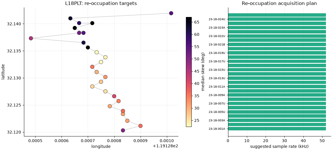
From an archive back to the field

In four steps an old EDI survey became a concrete IoT re-deployment: station geometry recovered, nodes provisioned with sensible sample rates, and a single QC standard tying the field crew’s edge decisions to the office processing. The forward bridge (edge impedance to a Z and an EDI) closes the loop on the next campaign.