
Note
Go to the end to download the full example code.
IoT field session: simulated telemetry, edge QC, and provenance#
This example is fully self-contained: it needs no field files and runs
anywhere. It uses the pycsamt.iot simulator to stand in for a real
IoT-enabled AMT deployment, then walks the operational lifecycle end to
end:
run AMT-specific edge QC on raw channel waveforms (powerline harmonics, SNR, resolvable frequency band, sensor dropout);
assemble a
FieldSessionfrom a station network, assess telemetry quality, and produce the processing hand-off;audit clock synchronisation (offset, drift, jitter, GPS lock); and
export a reproducible provenance bundle.
The companion example, IoT dashboard from bundled AMT station files, shows the same layer driven from real EDI inventory instead of the simulator.
1. Edge QC on simulated station waveforms#
simulate_amt_station returns per-channel time series plus ready-made
telemetry packets. We build a clean station and a powerline-contaminated
one (with dropouts), then let the AMT edge diagnostics tell them apart —
the boolean flags and resolved band are what make the IoT layer
scientifically meaningful.
from __future__ import annotations

import tempfile
from pathlib import Path

import matplotlib.pyplot as plt
import numpy as np

from pycsamt.iot import (
    ClockSynchronizer,
    FieldSession,
    SyncConfig,
    amt_edge_report,
    amt_edge_table,
    compute_live_spectra,
    detect_powerline_harmonics,
    detect_sensor_dropout,
    estimate_frequency_coverage,
    export_reproducibility_bundle,
    plot_edge_qc_summary,
    plot_field_dashboard,
    plot_sync_quality,
    simulate_amt_station,
    simulate_gps_drift,
    simulate_iot_network,
    sync_status_table,
)

SAMPLE_RATE = 256.0
MAINS_HZ = 50.0

clean = simulate_amt_station(
    "S001",
    channels=["ex", "ey", "hx", "hy"],
    sample_rate=SAMPLE_RATE,
    n_samples=4096,
    mains_hz=MAINS_HZ,
    snr_db=24.0,
    powerline_amplitude=0.0,
    dropout_rate=0.0,
    seed=11,
)
noisy = simulate_amt_station(
    "S002",
    channels=["ex", "ey", "hx", "hy"],
    sample_rate=SAMPLE_RATE,
    n_samples=4096,
    mains_hz=MAINS_HZ,
    snr_db=12.0,
    powerline_amplitude=0.6,
    dropout_rate=0.04,
    seed=12,
)

reports = {
    "S001 (clean)": amt_edge_report(
        clean["data"]["ex"], SAMPLE_RATE, mains_hz=MAINS_HZ
    ),
    "S002 (noisy)": amt_edge_report(
        noisy["data"]["ex"], SAMPLE_RATE, mains_hz=MAINS_HZ
    ),
}
qc_table = amt_edge_table(reports, api=False)
print(
    qc_table[
        [
            "channel",
            "powerline_contaminated",
            "powerline_total_ratio",
            "dropout",
            "nan_fraction",
            "f_low_hz",
            "f_high_hz",
        ]
    ].to_string(index=False)
)

ex = noisy["data"]["ex"]
harmonics = detect_powerline_harmonics(ex, SAMPLE_RATE, mains_hz=MAINS_HZ)
coverage = estimate_frequency_coverage(ex, SAMPLE_RATE)
dropout = detect_sensor_dropout(ex)
print(
    f"\nS002 Ex: mains contaminated={harmonics.contaminated}"
    f" (dominant {harmonics.dominant.frequency_hz:.0f} Hz,"
    f" ratio={harmonics.total_ratio:.2f})"
    f" | dropout={dropout['dropout']} (nan={dropout['nan_fraction']:.1%})"
    f" | resolved band {coverage.f_low_hz:.1f}-{coverage.f_high_hz:.1f} Hz"
)
     channel  powerline_contaminated  powerline_total_ratio  dropout  nan_fraction  f_low_hz  f_high_hz
s001 (clean)                   False               0.000167    False      0.000000       1.0       48.0
s002 (noisy)                    True               0.166247     True      0.039062       1.0      107.0

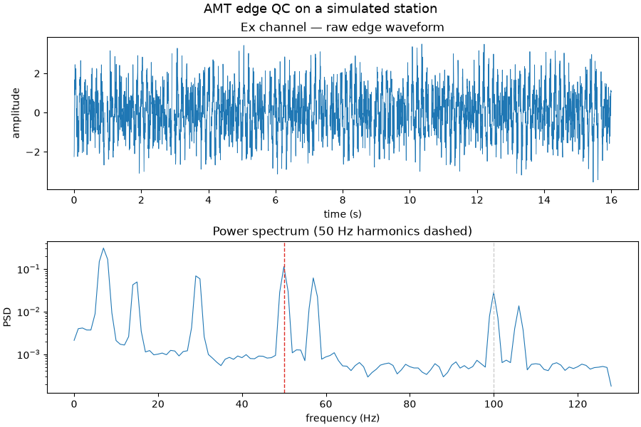
S002 Ex: mains contaminated=True (dominant 50 Hz, ratio=0.17) | dropout=True (nan=3.9%) | resolved band 1.0-107.0 Hz
The raw waveform and its spectrum make the contamination obvious: the dashed red lines mark powerline harmonics flagged by the detector.
spectrum = compute_live_spectra(ex, SAMPLE_RATE)
fig, (ax_time, ax_freq) = plt.subplots(
    2, 1, figsize=(9.0, 6.0), constrained_layout=True
)
time_s = np.arange(ex.size) / SAMPLE_RATE
ax_time.plot(time_s, ex, lw=0.6, color="#1f77b4")
ax_time.set(
    title="Ex channel — raw edge waveform",
    xlabel="time (s)",
    ylabel="amplitude",
)
ax_freq.semilogy(
    spectrum["frequency_hz"], spectrum["psd"] + 1e-12, lw=0.8, color="#1f77b4"
)
for peak in harmonics.peaks:
    ax_freq.axvline(
        peak.frequency_hz,
        color="#de2d26" if peak.flagged else "#cccccc",
        ls="--",
        lw=1.0,
    )
ax_freq.set(
    title=f"Power spectrum ({MAINS_HZ:.0f} Hz harmonics dashed)",
    xlabel="frequency (Hz)",
    ylabel="PSD",
)
fig.suptitle("AMT edge QC on a simulated station", fontsize=13)
Text(0.5, 0.993055, 'AMT edge QC on a simulated station')
2. Assemble a field session and assess the network#
simulate_iot_network emits health and QC packets for a fleet of
stations across two profiles. The session ingests them, grades the
stream, and produces a processing hand-off keyed by station.
packets = simulate_iot_network(
    n_stations=18,
    profiles=["L1", "L3"],
    channels=["ex", "ey", "hx", "hy"],
    sample_rate=SAMPLE_RATE,
    dropout_rate=0.02,
    survey_id="SIM-SURVEY",
    seed=7,
)
session = FieldSession("SIM-SURVEY", method="amt")
session.add_packets(packets)

status = session.assess()
print(status)
pipeline = session.to_pipeline_input()
print(
    f"pipeline hand-off: {pipeline['n_stations']} stations, "
    f"method={pipeline['method']}"
)

plot_field_dashboard(
    session,
    station_axis="profile",
    title="Simulated AMT survey - IoT field dashboard",
)
plot_edge_qc_summary(session, title="Simulated survey - edge QC telemetry")
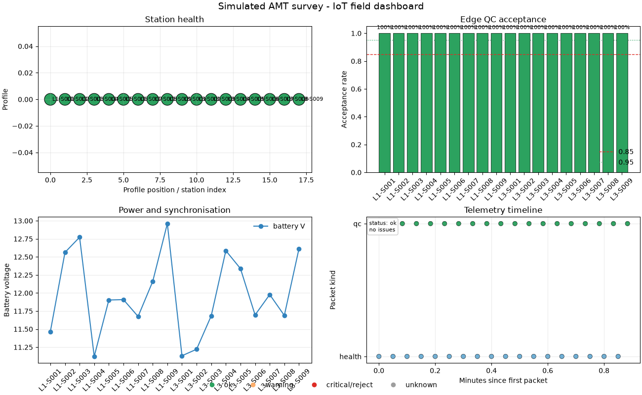
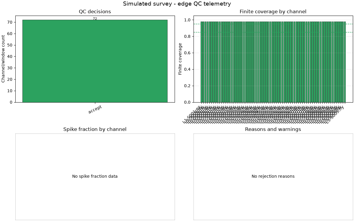
MonitoringStatus(level=<MonitoringLevel.OK: 'ok'>, n_packet=36, packet_success_rate=1.0, edge_acceptance_rate=1.0, mean_latency_s=nan, max_gap_s=2.0, battery_min_v=11.122, clock_offset_max_ms=nan, methods=['amt', 'unknown'], stations=['L1-S001', 'L1-S002', 'L1-S003', 'L1-S004', 'L1-S005', 'L1-S006', 'L1-S007', 'L1-S008', 'L1-S009', 'L3-S001', 'L3-S002', 'L3-S003', 'L3-S004', 'L3-S005', 'L3-S006', 'L3-S007', 'L3-S008', 'L3-S009'], channels=['ex', 'ey', 'hx', 'hy'], frequency_min_hz=1.0, frequency_max_hz=128.0, issues=[])
pipeline hand-off: 18 stations, method=amt

<Figure size 1200x750 with 4 Axes>
3. Clock-synchronisation audit#
simulate_gps_drift produces paired reference/local clocks with a set
drift and jitter; the last node also loses GPS lock. The synchroniser
grades each device on offset, drift, jitter, and lock state.
synchronizer = ClockSynchronizer(
    SyncConfig(tolerance_ms=2.0, max_drift_ppm=10.0)
)
sync_statuses = []
for index, drift_ppm in enumerate([3.0, 7.0, 22.0], start=1):
    clocks = simulate_gps_drift(
        240,
        sample_interval_s=1.0,
        drift_ppm=drift_ppm,
        jitter_ms=0.05,
        dropout_rate=0.0 if index < 3 else 0.25,
        seed=100 + index,
    )
    sync_statuses.append(
        synchronizer.assess(
            f"node-{index:02d}",
            clocks["local"],
            clocks["reference"],
            gps_lock=bool(clocks["gps_lock"].all()),
        )
    )

print(
    sync_status_table(sync_statuses, api=False)[
        [
            "device_id",
            "offset_ms",
            "drift_ppm",
            "jitter_ms",
            "quality",
            "within_tolerance",
        ]
    ].to_string(index=False)
)

plot_sync_quality(
    sync_statuses,
    tolerance_ms=2.0,
    title="Simulated fleet - clock synchronisation",
)
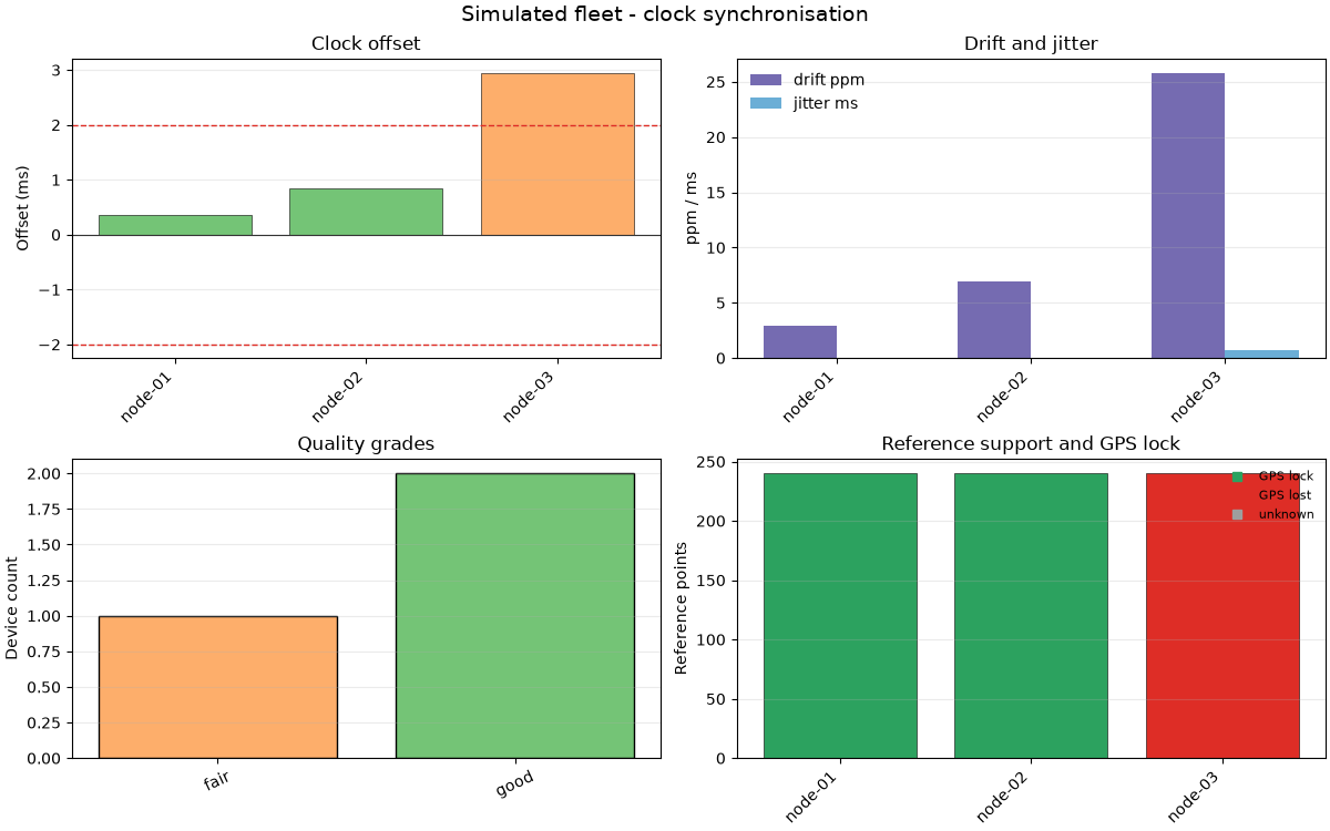
device_id  offset_ms  drift_ppm  jitter_ms quality  within_tolerance
  node-01   0.357628   2.965061   0.051935    good              True
  node-02   0.851989   6.935387   0.052351    good              True
  node-03   2.951741  25.769711   0.706183    fair             False

<Figure size 1200x750 with 4 Axes>
4. Export a reproducible provenance bundle#
The manifest records devices, per-station QC decisions, and a content hash; the bundle writes the manifest plus one audit file per station into a directory that can travel beside the raw data.
bundle_dir = Path(tempfile.mkdtemp()) / "sim_survey_reproducibility"
manifest = session.to_manifest()
bundle = export_reproducibility_bundle(manifest, str(bundle_dir))
print(f"manifest content hash: {manifest.as_dict()['content_hash'][:16]}...")
print(
    f"bundle: {Path(bundle['manifest']).name} "
    f"+ {len(bundle['audits'])} station audits"
)

plt.show()
manifest content hash: caf1d6e9c7ea9974...
bundle: acquisition_manifest.json + 18 station audits
Total running time of the script: (0 minutes 1.286 seconds)