Basic site loading and summary reporting

This first pycsamt.site gallery example answers a very practical question:

“I have EDI files on disk; what did pyCSAMT actually load?”

Before quality control, static-shift correction, inversion, or plotting, it is worth doing a lightweight site-level inspection. The goal is not to decide whether the survey is scientifically perfect. The goal is to verify the basic contract:

• every station you expect is visible;

• each station has a frequency vector;

• impedance components are present;

• coordinates and elevation were parsed when available;

• the apparent-resistivity and phase summaries look plausible enough to move to the next workflow.

The canonical entry point is pycsamt.emtools.ensure_sites(). It accepts an EDI file, a directory of EDI files, or an object that is already compatible with pycsamt.site.Sites, and returns a normalized Sites collection.

This page uses the bundled WILLY L18PLT line from data/AMT/WILLY_DATA. The same pattern applies to a project directory on your machine:

from pycsamt.emtools import ensure_sites

sites = ensure_sites("/path/to/my/edi_folder", recursive=True, verbose=0)

1. Imports and example-data location

Gallery scripts are executed by Sphinx, but users can also download and run them directly. During a docs build, docs/source/conf.py sets PYCSAMT_DOCS_REPO_ROOT. Outside the docs build, the path is inferred from this file location.

import os
import sys
from pathlib import Path

import matplotlib.pyplot as plt

from pycsamt.emtools import ensure_sites
from pycsamt.site.report import SitesReport


def repo_root() -> Path:
    """Return the repository root for bundled example data."""

    root = os.environ.get("PYCSAMT_DOCS_REPO_ROOT")
    return Path(root) if root else Path(__file__).resolve().parents[3]


ROOT = repo_root()
if str(ROOT) not in sys.path:
    sys.path.insert(0, str(ROOT))


edi_dir = ROOT / "data" / "AMT" / "WILLY_DATA" / "L18PLT"
print(f"Example EDI directory: {edi_dir}")

Example EDI directory: /opt/build/repo/data/AMT/WILLY_DATA/L18PLT

2. Load one survey line as a Sites collection

recursive=False is intentional here: L18PLT is already one station directory. For a parent folder that contains several survey lines, use recursive=True.

verbose=0 keeps gallery output compact. When exploring a new data drop, increasing verbosity can be useful while checking which files were accepted or skipped.

sites = ensure_sites(edi_dir, recursive=False, verbose=0)

print(type(sites).__name__)
print(f"Loaded station count: {len(sites)}")

Sites
Loaded station count: 28

A useful habit is to fail early if the loader returns an empty collection. Empty input usually means the path is wrong, files are not EDI files, or the EDI files do not contain valid impedance data.

if len(sites) == 0:
    raise RuntimeError(
        f"No stations with valid impedance were loaded from {edi_dir}"
    )

3. Build the high-level site report

SitesReport computes one record per station. It does not mutate the data. Think of it as a compact dashboard around the fields exposed by the site objects: frequency, impedance, apparent resistivity, phase, tipper, and header coordinates.

report = SitesReport(sites)
summary = report.to_dataframe()

print(report.summary())
print(summary.head(8).to_string(index=False))

SitesReport(28 stations  freq 1.008 Hz → 10.4 kHz)
station       lat        lon  elev  nfreq  freq_min  freq_max  has_Zxx  has_Zxy  has_Zyx  has_Zyy  has_tipper       rho_xy   rho_xy_std      rho_yx  rho_yx_std    phi_xy  phi_xy_std      phi_yx  phi_yx_std
18-013U 32.131083 119.128733 144.0     53     1.008   10400.0     True     True     True     True        True  5111.472834  7209.774419 1527.700407 1364.671531 14.282324   15.235792 -164.234813   10.133934
18-021U 32.138317 119.128683  52.0     53     1.008   10400.0     True     True     True     True        True  7836.120393  6938.888591 4132.650892 8067.376128 -1.399780   26.821366  -18.548028  144.999335
18-014A 32.132050 119.128717 125.0     53     1.008   10400.0     True     True     True     True        True 12938.810372 18041.194932  428.545253  471.445140  7.576143   13.693756 -149.942875   65.625954
18-006A 32.124767 119.128783 124.0     53     1.008   10400.0     True     True     True     True        True   974.817048  1169.034384  383.592596  411.905360 21.768599   15.337985 -156.388488    8.324562
18-010U 32.128417 119.128717 129.0     53     1.008   10400.0     True     True     True     True        True  5002.910700  6439.899679  267.890169  222.882674 18.198236   11.536741 -137.313086   24.038644
18-007U 32.125717 119.128817 126.0     53     1.008   10400.0     True     True     True     True        True  1391.634282  1781.248631 1093.874852 1497.389273 21.916802   15.040096 -147.599077   64.773804
18-016A 32.133817 119.128767  71.0     53     1.008   10400.0     True     True     True     True        True 15420.768297 19903.009307   61.345998   64.615767  9.365358   15.849129 -107.667760  116.255140
18-012A 32.130167 119.128767 126.0     53     1.008   10400.0     True     True     True     True        True  1333.182155  1898.757921  682.002234  545.701219 15.475271   15.654039 -142.768520   78.936284

The dataframe columns are intentionally plain and stable enough for quick checks in notebooks or tests.

station

Station name parsed from the EDI/header metadata.

lat, lon, elev

Location metadata when present.

nfreq, freq_min, freq_max

Number of frequency samples and each station’s frequency span.

has_Zxx … has_Zyy

Availability flags for impedance tensor components.

has_tipper

Whether tipper data are available.

rho_xy, rho_yx, phi_xy, phi_yx

Per-station summary statistics for the off-diagonal apparent resistivity and phase components.

print("Summary columns:")
print(", ".join(summary.columns))

Summary columns:
station, lat, lon, elev, nfreq, freq_min, freq_max, has_Zxx, has_Zxy, has_Zyx, has_Zyy, has_tipper, rho_xy, rho_xy_std, rho_yx, rho_yx_std, phi_xy, phi_xy_std, phi_yx, phi_yx_std

4. Station names and frequency coverage

The first check most users care about is whether the expected station names appear. Here we print a compact station list and the frequency-count range.

station_names = summary["station"].tolist()
print("First 10 station names:")
print(station_names[:10])

print(
    "Frequency rows per station:",
    int(summary["nfreq"].min()),
    "to",
    int(summary["nfreq"].max()),
)

print(
    "Overall frequency span:",
    f"{summary['freq_min'].min():.4g}",
    "to",
    f"{summary['freq_max'].max():.4g}",
    "Hz",
)

First 10 station names:
['18-013U', '18-021U', '18-014A', '18-006A', '18-010U', '18-007U', '18-016A', '18-012A', '18-005U', '18-017U']
Frequency rows per station: 53 to 53
Overall frequency span: 1.008 to 1.04e+04 Hz

5. Component availability

For most MT/AMT/CSAMT workflows, the off-diagonal components Zxy and Zyx are the workhorses. Diagonal components are also useful for diagnostics, dimensionality checks, and data quality interpretation.

component_columns = ["has_Zxx", "has_Zxy", "has_Zyx", "has_Zyy", "has_tipper"]
availability = summary[component_columns].sum().astype(int)

print("Component availability, counted by station:")
print(availability.to_string())

Component availability, counted by station:
has_Zxx       28
has_Zxy       28
has_Zyx       28
has_Zyy       28
has_tipper    28

If a component count is unexpectedly low, do not patch around it silently. Go back to the EDI source and confirm whether the component is genuinely missing, masked, or stored under a convention that needs a reader update.

required = ["has_Zxy", "has_Zyx"]
missing_required = {
    col: int((~summary[col]).sum())
    for col in required
    if col in summary and (~summary[col]).any()
}

if missing_required:
    print("Stations missing key off-diagonal components:", missing_required)
else:
    print("All loaded stations expose Zxy and Zyx.")

All loaded stations expose Zxy and Zyx.

6. A quick visual smoke test

Gallery examples should leave the reader with a visual intuition. This small figure is not a scientific interpretation; it is a quick smoke test: do all stations carry similar frequency counts, and is the line complete?

fig, ax = plt.subplots(figsize=(9, 3.6))
ax.bar(summary["station"], summary["nfreq"], color="#3b82f6")
ax.set_title("Frequency rows per station")
ax.set_xlabel("Station")
ax.set_ylabel("Number of frequencies")
ax.tick_params(axis="x", rotation=75)
ax.grid(axis="y", alpha=0.25)
fig.tight_layout()

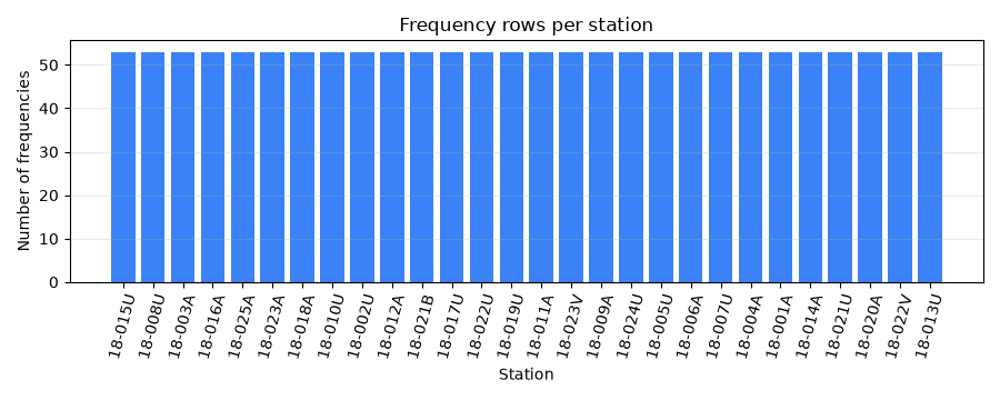
In a healthy line, this plot is usually boring: similar bar heights across stations. Boring is good here. A short bar is a station to inspect before heavier processing.

7. Use report dictionaries for lightweight automation

to_dataframe is convenient when pandas is available. to_dict is a simple list of Python dictionaries, which can be easier for lightweight checks, JSON serialization, or tests that should avoid dataframe-specific assertions.

records = report.to_dict()
first = records[0]

print("Keys available in one report record:")
print(sorted(first.keys()))

print("First station compact record:")
print(
    {
        "name": first["name"],
        "nfreq": first["nfreq"],
        "freq_min": first["freq_min"],
        "freq_max": first["freq_max"],
        "has_tipper": first["has_tipper"],
    }
)

Keys available in one report record:
['components', 'elev', 'freq_max', 'freq_min', 'has_tipper', 'lat', 'lon', 'name', 'nfreq', 'per_max', 'per_min', 'phi_xy_mean', 'phi_xy_std', 'phi_yx_mean', 'phi_yx_std', 'quality', 'rho_xy_mean', 'rho_xy_std', 'rho_yx_mean', 'rho_yx_std']
First station compact record:
{'name': '18-013U', 'nfreq': 53, 'freq_min': 1.008, 'freq_max': 10400.0, 'has_tipper': True}

8. Optional terminal report

SitesReport.report prints a human-readable panel. When rich is installed the output is formatted; otherwise pyCSAMT falls back to plain text. Limit the table with top when running in CI or documentation.

report.report(top=5)

╭───────────────────────────── Survey Summary ─────────────────────────────╮
│ Stations     28                                                          │
│ Coverage     Lat 32.12–32.14°N  ·  Lon 119.13–119.13°E  ·  Elev 37–144 m │
│ Frequencies  53–53 freq/station  ·  1.008 Hz → 10.4 kHz                  │
╰──────────────────────────────────────────────────────────────────────────╯
                               Stations (5 of 28)
┏━━━━━━━━━┳━━━━━━┳━━━━━━┳━━━━━━┳━━━━━━┳━━━━━━┳━━━━━━┳━━━━━━━━┳━━━━━━━━┳━━━━━━━━┓
┃         ┃      ┃      ┃      ┃      ┃      ┃      ┃   ρ_xy ┃        ┃        ┃
┃ Station ┃ Freq ┃ Zxx  ┃ Zxy  ┃ Zyx  ┃ Zyy  ┃ Tip  ┃    Ω·m ┃ φ_xy ° ┃ Cover  ┃
┡━━━━━━━━━╇━━━━━━╇━━━━━━╇━━━━━━╇━━━━━━╇━━━━━━╇━━━━━━╇━━━━━━━━╇━━━━━━━━╇━━━━━━━━┩
│ 18-013U │   53 │  ✓   │  ✓   │  ✓   │  ✓   │  ✓   │ 5111±… │ 14.3±… │ ██████ │
│ 18-021U │   53 │  ✓   │  ✓   │  ✓   │  ✓   │  ✓   │ 7836±… │ -1.4±… │ ██████ │
│ 18-014A │   53 │  ✓   │  ✓   │  ✓   │  ✓   │  ✓   │ 12939… │ 7.6±1… │ ██████ │
│ 18-006A │   53 │  ✓   │  ✓   │  ✓   │  ✓   │  ✓   │ 975±1… │ 21.8±… │ ██████ │
│ 18-010U │   53 │  ✓   │  ✓   │  ✓   │  ✓   │  ✓   │ 5003±… │ 18.2±… │ ██████ │
└─────────┴──────┴──────┴──────┴──────┴──────┴──────┴────────┴────────┴────────┘

╭───────── Component Availability ──────────╮
│ Zxx    ████████████████      28/28   100% │
│ Zxy    ████████████████      28/28   100% │
│ Zyx    ████████████████      28/28   100% │
│ Zyy    ████████████████      28/28   100% │
│ Tipper ████████████████      28/28   100% │
╰───────────────────────────────────────────╯

9. What this first example should tell you

After this page, the survey has passed only a loading and visibility check. That is still valuable. You now know the line can be represented as a Sites collection and that the summary statistics are accessible.

Recommended next steps:

• use the next site-gallery example to select/filter a robust subset;

• run pycsamt.emtools.qc for confidence scoring and failure flags;

• inspect static shift, dimensionality, strike, and phase-tensor diagnostics before inversion.