Frequency editing and EMAP denoising

Once the confidence diagnostics (see Frequency coverage and data-quality confidence) show where the data is weak, the next step is to act on it: recover or drop individual frequencies by confidence, and suppress spatially incoherent noise with an electromagnetic-array-profiling (EMAP) filter. This example runs both edits on line L22PLT, keeping an untouched baseline alongside each edited copy so the before/after figures are honest comparisons.

The editing routines live in pycsamt.emtools.frequency (confidence-driven frequency edits) and pycsamt.emtools.remove_noise (EMAP filtering and its confidence-gated variant).

Confidence-driven frequency editing

edit_frequencies_by_confidence() scores every (station, frequency) cell and, in "recover" mode, keeps high-confidence cells, attempts to recover marginal ones, and drops the rest. We load two independent copies of L22PLT — one frozen baseline, one to edit — so nothing leaks between them.

import logging
from contextlib import contextmanager

from _datasets import load_sites

from pycsamt.emtools.frequency import (
    edit_frequencies_by_confidence,
    plot_frequency_edit_decisions,
    plot_frequency_edit_summary,
)


@contextmanager
def quiet_recompute_logs():
    """Silence the impedance object's expected recompute diagnostics.

    Recover-mode editing masks rejected cells; setting the (now
    non-finite) Z then logs a "cannot recompute rho/phi" error per masked
    cell. Those are internal diagnostics, not failures — scope a global
    ``logging.disable`` around the edit so the example output stays
    readable without affecting any other gallery script.
    """
    logging.disable(logging.ERROR)
    try:
        yield
    finally:
        logging.disable(logging.NOTSET)


from pycsamt.emtools.remove_noise import (
    apply_emap_filter,
    confidence_gated_emap_filter,
    emap_filter_report,
    plot_emap_filter_profile,
    plot_emap_filter_psection,
)

before = load_sites("amt_l22plt")
source = load_sites("amt_l22plt")

with quiet_recompute_logs():
    edit = edit_frequencies_by_confidence(
        source,
        before_sites=before,
        mode="recover",
        method="composite",
        ci_hi=0.90,
        ci_lo=0.50,
        reject="drop",
    )

# The edit returns a per-cell decision table and a per-station report —
# inspect them just as you would on your own data.
print("report columns:", list(edit.report.columns))
print(edit.report.head().to_string(index=False))
print("\ndecision table columns:", list(edit.decisions.columns))
print(edit.decisions.head().to_string(index=False))

report columns: ['station', 'n_freq_before', 'n_finite_before', 'frac_finite_before', 'n_freq_after', 'n_finite_after', 'frac_finite_after', 'confidence_median_before', 'safe_fraction_before', 'recoverable_fraction_before', 'reject_fraction_before', 'confidence_median_after', 'safe_fraction_after', 'recoverable_fraction_after', 'reject_fraction_after', 'n_dropped', 'n_masked_or_unfinite', 'confidence_delta']
 station  n_freq_before  n_finite_before  frac_finite_before  n_freq_after  n_finite_after  frac_finite_after  confidence_median_before  safe_fraction_before  recoverable_fraction_before  reject_fraction_before  confidence_median_after  safe_fraction_after  recoverable_fraction_after  reject_fraction_after  n_dropped  n_masked_or_unfinite  confidence_delta
22-013VF             53               53                 1.0            53               0                0.0                  0.765127                   0.0                     1.000000                0.000000                      0.0                  0.0                         0.0                    1.0          0                    53         -0.765127
22-025AF             53               53                 1.0            43               0                0.0                  0.553056                   0.0                     0.811321                0.188679                      0.0                  0.0                         0.0                    1.0         10                    53         -0.553056
  22-10U             53               53                 1.0            52               0                0.0                  0.771960                   0.0                     0.981132                0.018868                      0.0                  0.0                         0.0                    1.0          1                    53         -0.771960
  22-11A             53               53                 1.0            52               0                0.0                  0.607969                   0.0                     0.981132                0.018868                      0.0                  0.0                         0.0                    1.0          1                    53         -0.607969
  22-12U             53               53                 1.0            48               0                0.0                  0.617632                   0.0                     0.905660                0.094340                      0.0                  0.0                         0.0                    1.0          5                    53         -0.617632

decision table columns: ['station', 'frequency_hz', 'period_s', 'log10_period', 'confidence', 'flags', 'finite_before', 'present_after', 'finite_after', 'action']
station  frequency_hz  period_s  log10_period  confidence                       flags  finite_before  present_after  finite_after action
 22-2VF       10400.0  0.000096     -4.017033    0.767565 recoverable,spatial_outlier           True           True         False masked
 22-2VF        8707.0  0.000115     -3.939869    0.776846 recoverable,spatial_outlier           True           True         False masked
 22-2VF        7289.0  0.000137     -3.862668    0.764411 recoverable,spatial_outlier           True           True         False masked
 22-2VF        6102.0  0.000164     -3.785472    0.750194 recoverable,spatial_outlier           True           True         False masked
 22-2VF        5108.0  0.000196     -3.708251    0.755739 recoverable,spatial_outlier           True           True         False masked

1. Edit summary

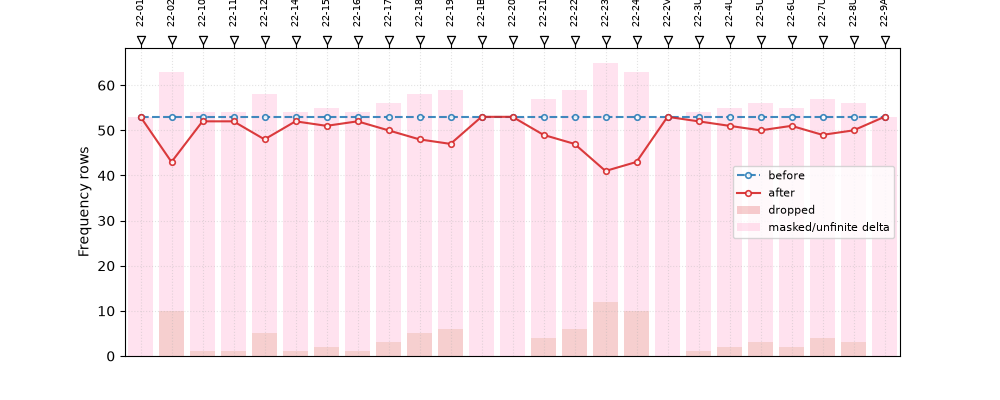
plot_frequency_edit_summary() contrasts the confidence distribution before and after the edit, so you can confirm the operation improved the line as a whole.

plot_frequency_edit_summary(
    before,
    edit.sites,
    method="composite",
    ci_hi=0.90,
    ci_lo=0.50,
    figsize=(10, 4.0),
)

<Axes: title={'center': 'Frequency edit summary'}, xlabel='Station', ylabel='Frequency rows'>

2. Per-cell edit decisions

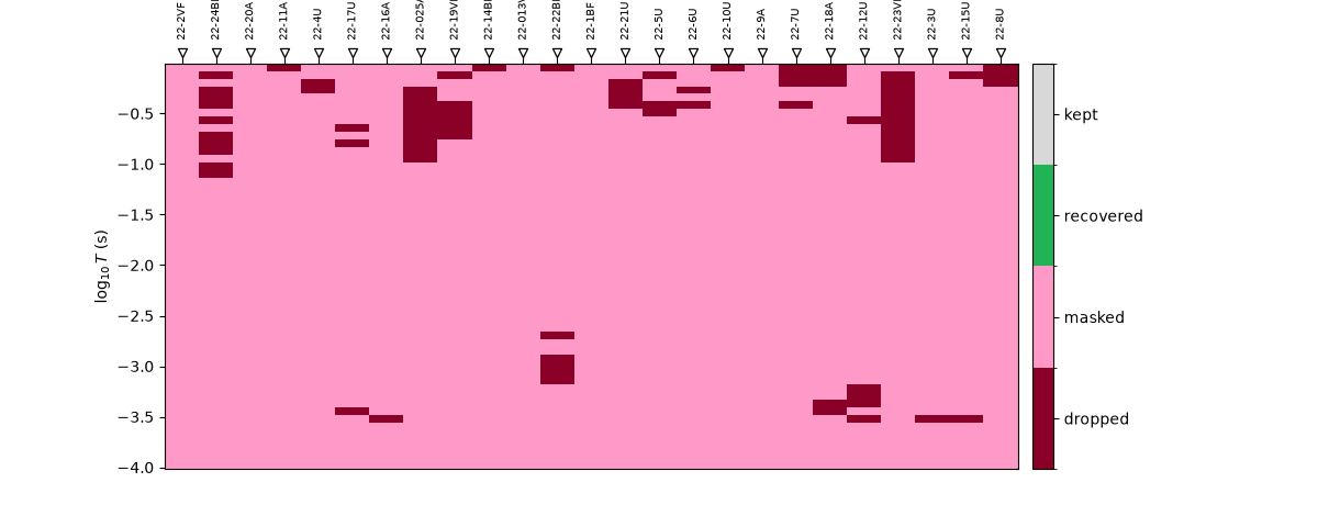
plot_frequency_edit_decisions() maps the actual keep / recover / drop decision onto the station-by-period grid — a precise audit of what the edit changed and where.

plot_frequency_edit_decisions(
    before,
    edit.sites,
    method="composite",
    ci_hi=0.90,
    ci_lo=0.50,
    figsize=(12, 4.8),
)

<Axes: title={'center': 'Frequency edit decisions'}, xlabel='Station', ylabel='$\\log_{10}T$ (s)'>

EMAP FLMA denoising

apply_emap_filter() applies a first-order moving-average (FLMA) EMAP filter along the profile, averaging each station’s response with its neighbours to suppress static and spatially random noise on the xy component.

emap_before = load_sites("amt_l22plt")
emap_source = load_sites("amt_l22plt")
flma = apply_emap_filter(emap_source, method="flma", window=5, component="xy")

report = emap_filter_report(
    emap_before,
    flma,
    component="xy",
    period_s=0.01,
)
print(report.head().to_string(index=False))

station component  n_matched_freq  median_delta_log10_abs_z  rms_delta_log10_abs_z  reference_frequency_hz  reference_frequency_after_hz  before_log10_abs_z  after_log10_abs_z  reference_delta_log10_abs_z
 22-2VF        xy              53                  0.222564               0.265978                   102.4                         102.4            2.382263           2.443190                     0.060927
22-24BF        xy              53                 -0.066073               0.100143                   102.4                         102.4            2.569363           2.528648                    -0.040715
 22-20A        xy              53                 -0.095288               0.154929                   102.4                         102.4            2.355659           2.520622                     0.164963
 22-11A        xy              53                 -0.003629               0.164350                   102.4                         102.4            2.738359           2.696204                    -0.042155
  22-4U        xy              53                  0.336267               0.334541                   102.4                         102.4            2.487987           2.753594                     0.265607

3. Filter effect on one station profile

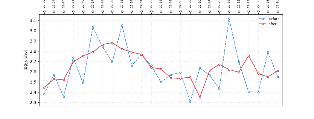
plot_emap_filter_profile() overlays the raw and filtered apparent resistivity along the line at a fixed period, showing how much smoothing the window applies.

plot_emap_filter_profile(
    emap_before,
    flma,
    method="flma",
    component="xy",
    period_s=0.01,
    figsize=(10.5, 4.0),
)

<Axes: title={'center': 'FLMA profile at 102.4 Hz'}, xlabel='Station', ylabel='$\\log_{10}|Z_{XY}|$'>

4. Before / after pseudo-section

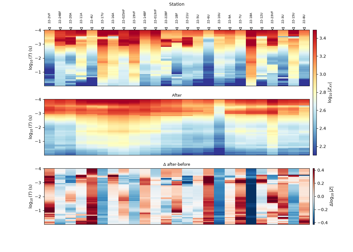
plot_emap_filter_psection() gives the full-band picture: raw and FLMA-filtered pseudo-sections side-by-side over every station and period.

plot_emap_filter_psection(
    emap_before,
    flma,
    method="flma",
    component="xy",
    figsize=(11.5, 8.2),
)

<Figure size 1150x820 with 5 Axes>

5. Confidence-gated EMAP

confidence_gated_emap_filter() combines both ideas: it only lets the FLMA filter modify low-confidence cells, leaving trustworthy data untouched. This is the recommended denoiser — it cleans the noisy corners of the band without smearing the parts that were already good.

gated_before = load_sites("amt_l22plt")
gated_source = load_sites("amt_l22plt")
with quiet_recompute_logs():
    gated = confidence_gated_emap_filter(
        gated_source,
        before_sites=gated_before,
        method="flma",
        confidence_method="composite",
        component="xy",
        window=5,
        ci_hi=0.90,
        ci_lo=0.50,
    )
print("gated decision table columns:", list(gated.decisions.columns))
print(gated.decisions.head().to_string(index=False))

plot_emap_filter_psection(
    gated_before,
    gated.sites,
    method="confidence-gated FLMA",
    component="xy",
    figsize=(11.5, 8.2),
)

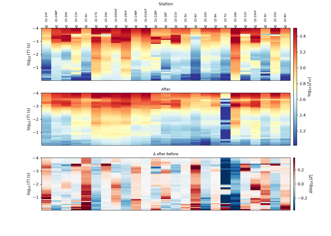
gated decision table columns: ['station', 'frequency_hz', 'period_s', 'log10_period', 'confidence', 'blend_weight', 'action', 'delta_log10_abs_z']
station  frequency_hz  period_s  log10_period  confidence  blend_weight  action  delta_log10_abs_z
 22-2VF       10400.0  0.000096     -4.017033    0.767565      0.331087 blended           0.066557
 22-2VF        8707.0  0.000115     -3.939869    0.776846      0.307884 blended           0.061284
 22-2VF        7289.0  0.000137     -3.862668    0.764411      0.338972 blended           0.072284
 22-2VF        6102.0  0.000164     -3.785472    0.750194      0.374515 blended           0.094629
 22-2VF        5108.0  0.000196     -3.708251    0.755739      0.360653 blended           0.098883

<Figure size 1150x820 with 5 Axes>