Geoelectric strike analysis

The geoelectric strike — the preferred 2-D structural axis inferred from the impedance tensor — ties the whole survey together. This example estimates and visualises it across the WILLY_DATA AMT survey using pycsamt.emtools.strike: per-station map-sticks and along-line profiles on L22PLT, a five-panel rose comparison across all profile lines, a short-vs-long-period band decomposition, and a strike ribbon.

Strike from all five lines together is what reveals whether the survey area shares one regional structural grain or breaks into domains — the kind of conclusion a single line cannot support.

1. Strike map-sticks (L22PLT)

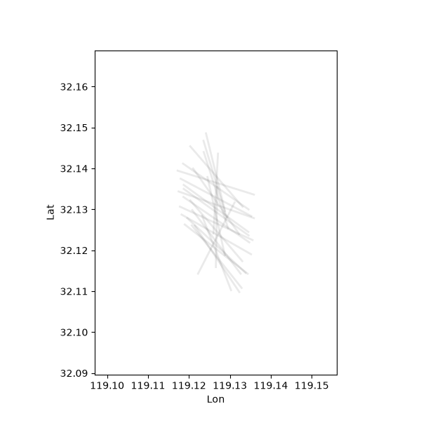
plot_strike_mapsticks() places a short oriented stick at each station’s map position, pointing along its estimated strike — the most literal way to see strike vary in space. (WILLY_DATA has no tipper, so this replaces the induction-arrow map that would otherwise accompany it; see Tipper and induction arrows for real induction vectors on KAP03.)

from _datasets import line_groups, load_sites

from pycsamt.emtools.strike import (
    plot_strike_mapsticks,
    plot_strike_profile,
    plot_strike_ribbon,
    plot_strike_rose,
)
from pycsamt.emtools.tensor import plot_theta_rose_grid

L22 = load_sites("amt_l22plt")

plot_strike_mapsticks(L22, method="consensus", figsize=(6, 6))

<Axes: xlabel='Lon', ylabel='Lat'>

2. Strike roses across all five lines

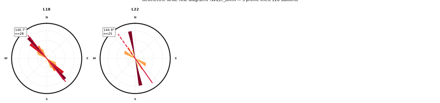
plot_strike_rose() draws one axial rose per profile line, side-by-side, from the full 128-station survey. A shared, dominant orientation across panels is evidence of a single regional strike.

S_all = load_sites("amt_willy", recursive=True)
groups = line_groups(S_all)

plot_strike_rose(
    S_all,
    groups=groups,
    method="consensus",
    bins=24,
    bar_style="gradient",
    cmap="YlOrRd",
    outer_ring_lw=2.5,
    outer_ring_color="0.12",
    n_rings=3,
    spoke_every=45.0,
    compass_labels="NESW",
    compass_fontsize=7.5,
    mean_color="crimson",
    mean_lw=2.2,
    show_secondary=True,
    secondary_ls="--",
    annotation_fontsize=8.0,
    show_n_stations=True,
    subplot_size=3.0,
    n_cols=5,
    suptitle="Geoelectric strike rose diagrams  "
    "(WILLY_DATA — 5 profile lines, 128 stations)",
    suptitle_fontsize=10,
)

<Figure size 1540x360 with 2 Axes>

3. Strike rose by period band (L22PLT)

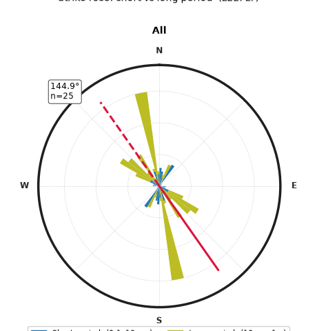
The same function with bar_style="bands" splits one line’s strike into short- and long-period contributions. A strike that rotates with period is a classic sign of a shallow structural grain overprinting a different deep one.

plot_strike_rose(
    L22,
    bar_style="bands",
    freq_bands=[(1e-4, 1e-2), (1e-2, 1e0)],
    band_labels=["Short period  (0.1–10 ms)", "Long period  (10 ms–1 s)"],
    bins=24,
    outer_ring_lw=2.5,
    outer_ring_color="0.12",
    spoke_every=45.0,
    compass_labels="NESW",
    annotation_fontsize=8.5,
    show_n_stations=True,
    subplot_size=4.2,
    suptitle="Strike rose: short vs long period  (L22PLT)",
    suptitle_fontsize=10,
)

<Figure size 460x480 with 1 Axes>

4. Strike colour ribbon

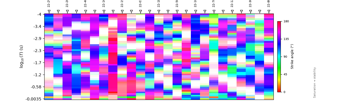
plot_strike_ribbon() shows strike as a colour band over station and log-period, exposing per-frequency detail the roses average away.

plot_strike_ribbon(L22, method="sweep", figsize=(12, 3.8))

<Axes: xlabel='Station', ylabel='$\\log_{10}(T)$ (s)'>

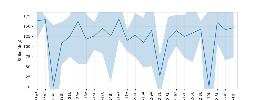
5. Strike profile along the line

plot_strike_profile() reduces strike to a median-plus-IQR trend along the stations — the compact summary to carry into an inversion mesh design.

plot_strike_profile(L22, method="consensus", figsize=(10, 3.8))

<Axes: xlabel='Station', ylabel='Strike (deg)'>

6. Phase-tensor strike rose grid by decade

plot_theta_rose_grid() cross-checks the strike estimate against the phase tensor directly, one rose per frequency decade — an independent view of the same directional information.

plot_theta_rose_grid(L22)

<Figure size 1300x380 with 6 Axes>