Geoelectric strike director field

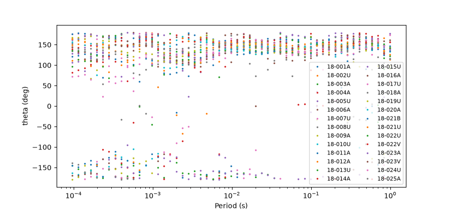
Phase-tensor strike theta is an axial angle — it is defined only up to 180°, so 179° is one degree from 0°, not 179 away. Plotting it on a linear axis (plot_theta_vs_period()) breaks at that wrap and collapses every station onto one crowded axis. The director field (plot_strike_director_field()) is a supplement built for the geometry of the quantity: it draws the strike as a direction at every station and depth at once, and folds in how much that direction can be trusted.

This example works through it as an interpretation tool on the WILLY_DATA survey and a long-period MT line, and shows the option knobs.

The problem: a linear strike scatter

The conventional view scatters raw strike against period for every station. It answers “is strike stable with depth?” but the axial wrap and the station pile-up make lateral structure impossible to read.

from _datasets import load_sites

from pycsamt.emtools.tensor import (
    plot_strike_director_field,
    plot_theta_vs_period,
)

L18 = load_sites("amt_l18plt")  # 28 stations, real error tensors
plot_theta_vs_period(L18, figsize=(9, 4.2))

<Axes: xlabel='Period (s)', ylabel='theta (deg)'>

The director field

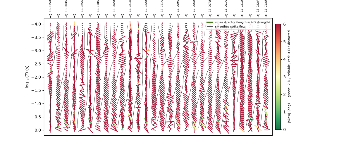
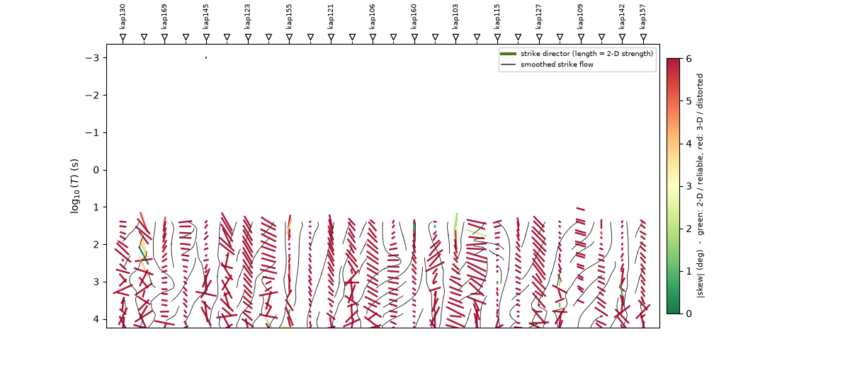
Each (station, period) cell becomes a head-less bar oriented along the strike (head-less because strike has no forward direction). Two more channels ride along:

• length = ellipticity (2-D strength) — near-1-D cells shrink toward a dot, because there the strike is genuinely ill-defined;

• colour = |skew| (distortion) — green where the strike is a reliable 2-D reading, red where 3-D / galvanic distortion makes it untrustworthy.

The smoothed streamline overlay integrates the bars into a strike “flow”, so coherence reads at a glance.

plot_strike_director_field(L18, figsize=(12, 5.2))

<Axes: title={'center': 'Geoelectric strike director field'}, xlabel='Station', ylabel='$\\log_{10}(T)$ (s)'>

How to read it

The picture tells you both the strike and how much to believe it:

• long, aligned, green bars in a laminar bundle → robust, depth-consistent 2-D strike; read the azimuth with confidence;

• bars rotating smoothly with depth → strike changes with depth (dipping structure or layered anisotropy);

• short and/or red, swirling bars → 1-D, 3-D, or noise: do not over-interpret the direction.

On L18PLT the field is dominated by red — the honest verdict, matching the strong 3-D / galvanic character this line shows in its skew and static-shift behaviour. Crucially the plot does not hide that: it flags the unreliability in colour while the streamlines still recover the coherent dominant azimuth, and the few long green bars mark the cells where a 2-D interpretation is defensible.

Colour by anisotropy instead of distortion

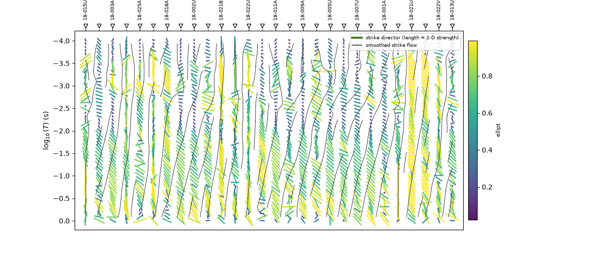
color_by accepts any table column. Colouring by ellipticity highlights where the 2-D signal is strongest rather than where it is distorted — a complementary read of the same field.

plot_strike_director_field(
    L18,
    color_by="ellipt",
    cmap="viridis",
    figsize=(12, 5.2),
    title="Strike director field — coloured by 2-D strength (L18PLT)",
)

<Axes: title={'center': 'Strike director field — coloured by 2-D strength (L18PLT)'}, xlabel='Station', ylabel='$\\log_{10}(T)$ (s)'>

A pure orientation field

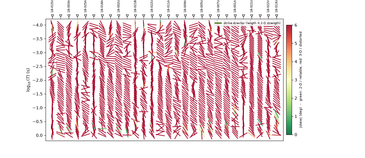
Setting length_by=None gives every bar the same length (orientation only) and streamlines=False strips the overlay — the barest, cleanest “which way does strike point” view, useful when ellipticity is nearly uniform.

plot_strike_director_field(
    L18,
    length_by=None,
    streamlines=False,
    figsize=(12, 5.2),
    title="Pure strike-orientation field (L18PLT)",
)

<Axes: title={'center': 'Pure strike-orientation field (L18PLT)'}, xlabel='Station', ylabel='$\\log_{10}(T)$ (s)'>

A long-period MT line

The same tool on KAP03, a SAMTEX long-period MT line with a very different (deeper) period band. The streamline overlay automatically confines itself to the populated period band, so it never invents flow in the empty short-period region.

KAP = load_sites("mt_kap03")
plot_strike_director_field(
    KAP,
    figsize=(12, 5.2),
    title="Strike director field (KAP03)",
)

<Axes: title={'center': 'Strike director field (KAP03)'}, xlabel='Station', ylabel='$\\log_{10}(T)$ (s)'>

Takeaway. The director field is the axial-aware companion to the strike scatter and the phase-tensor ellipses: it is the only view that shows strike as a direction over space and depth with a built-in reliability channel. Use it first to decide where a 2-D strike is worth reading, then read the azimuth from the rose (Phase-tensor ellipses) or rotate to strike for 2-D inversion.