
18.21. Interpret A Two-Line Occam2D Survey With interp And geology#
Build A Two-Line Occam2D Survey For Interpretation produced two real, independently
inverted resistivity sections – Line A and Line B, each crossing the
same kind of dipping fault at a different angle. Both sections show only
a broad, smooth resistivity tilt; neither shows the fault itself as a
sharp feature, because smoothness-regularized Occam2D is not built to
reproduce a discrete offset that way. This page is what turns those two
smooth images into an actual geological interpretation: calibrate each
one against a pair of boreholes, classify the calibrated model into
lithology with pycsamt.geology, record the fault as independent
structural evidence rather than expecting to read it off the resistivity
image, and then – honestly – check the result against two more
boreholes that were not used for calibration.
Every real number below comes from the same real Occam2D results Part 1
produced (loaded fresh, not re-inverted) and from the same true earth
model, queried directly with
value_at() for borehole ground
truth – the same function, the same coordinate convention, used
consistently from the forward model all the way through validation.
18.21.1. A project-specific rock table#
The built-in default() table is a
literature compilation, not tuned to any one site –
Rock resistivity database already shows the same query
value classified differently by two different tables. Classifying this
survey’s own true resistivities (80, 300, 3000 Ω·m) against the built-in
table returns “Fractured zone”, “Granite (weathered)”, and “Dolomite” –
geologically plausible names, but not the actual overburden / weathered
basement / fresh basement sequence this survey’s own boreholes describe.
A small regional table, built the same way
Rock resistivity database demonstrates, fixes that:
>>> from pycsamt.geology import RockDatabase, RockEntry
>>> regional_db = RockDatabase([
...     RockEntry(name="Overburden", rho_min=30, rho_max=180,
...               color="#D4AC0D", source="Site-specific, this survey"),
...     RockEntry(name="Weathered basement", rho_min=180, rho_max=900,
...               color="#A9780C", source="Site-specific, this survey"),
...     RockEntry(name="Fresh basement", rho_min=900, rho_max=8000,
...               color="#4A4A4A", source="Site-specific, this survey"),
... ])
>>> [regional_db.classify(rho).name for rho in (80.0, 300.0, 3000.0)]
['Overburden', 'Weathered basement', 'Fresh basement']
18.21.2. Boreholes, sampled honestly from the true model#
Every borehole below is built the same way: read the true earth model
Part 1 built – not the inversion, not a guess – at a chosen profile
position, with value_at(), exactly
as a real drilling program would measure it. Four boreholes per line,
split two ways: two for calibration, two held out entirely for
validation later on this page.
>>> from pycsamt.geology import Borehole, Interval
>>> from pycsamt.forward.synthetic import LayeredModel
>>> from pycsamt.forward.grid2d import Grid2D

>>> true_layers = LayeredModel(resistivity=[80.0, 300.0, 3000.0], thickness=[60.0, 260.0])
>>> grid_a = Grid2D.layered_with_fault(
...     true_layers, fault_x_m=1200.0, apparent_dip_deg=65.0,
...     throw_m=700.0, downthrown_side="right",
...     nx=60, nz=50, x_max=2400.0, z_max=1600.0, n_stations=25, name="Line A",
... )
Scanning depth at a fixed x and recording every resistivity change
gives the real interval boundaries – close to, but not exactly, the
nominal 60/320 m layer depths, since a real log is quantised by the
grid’s own cell size just as a real logging tool has finite sample
spacing:
>>> import numpy as np
>>> def true_intervals(grid, x_m, max_depth_m, dz=1.0):
...     zs = np.arange(0.0, max_depth_m + dz, dz)
...     vals = np.array([grid.value_at(x_m, z, chainage=True) for z in zs])
...     out, start = [], 0
...     for i in range(1, len(zs)):
...         if vals[i] != vals[i - 1]:
...             out.append((float(zs[start]), float(zs[i]), float(vals[i - 1])))
...             start = i
...     out.append((float(zs[start]), float(zs[-1]), float(vals[-1])))
...     return out

>>> true_intervals(grid_a, 300.0, 450.0)
[(0.0, 65.0, 80.0), (65.0, 321.0, 300.0), (321.0, 450.0, 3000.0)]
Wrapping each interval in this way, with the true resistivity carried
alongside the lithology name classified against regional_db,
produces the actual Borehole objects the
calibrator – and, later, the validation step – will use:
>>> def borehole_from_true(grid, name, x_m, max_depth_m):
...     ivs = [
...         Interval(top=top, bottom=bottom, resistivity=rho,
...                  lithology=regional_db.classify(rho).name)
...         for top, bottom, rho in true_intervals(grid, x_m, max_depth_m)
...     ]
...     return Borehole(name, x=x_m, intervals=ivs)

>>> bh_a1 = borehole_from_true(grid_a, "A1", 300.0, 450.0)
>>> bh_a2 = borehole_from_true(grid_a, "A2", 2100.0, 1100.0)
>>> [iv.lithology for iv in bh_a1.intervals]
['Overburden', 'Weathered basement', 'Fresh basement']
A1 (footwall, x=300 m) only needs to reach 450 m to confirm fresh
basement; A2 (downthrown, x=2100 m) needs 1100 m for the same
confirmation, because the same basement contact sits roughly 700 m
deeper there – a direct, physical consequence of the fault throw, not
an arbitrary choice. Both calibration boreholes sit comfortably inside
the footwall or downthrown block at every depth drilled – the fault
plane itself migrates with depth (x = fault_x + z / tan(apparent_dip)),
and a borehole placed too close to the surface trace can cross from one
side to the other partway down, which would make “the true log at this
x” ambiguous. A1, A2, and the two validation boreholes below were all
checked against that migration and kept clear of it; Structural measurements
covers the general apparent-dip geometry this follows.
The two validation boreholes – A3 (footwall, x=900 m) and A4
(downthrown, x=1800 m) – are built exactly the same way, but are never
passed to the calibrator. Line B’s four boreholes mirror this with its
own fault geometry (downthrown_side="left"): B1/B2 for
calibration at x=300/1900 m, B3/B4 held out at x=100/2100 m.
18.21.3. See every borehole at a glance#
Before any of these boreholes touch the inversion, it helps to look at
all four on a line side by side – exactly the raw evidence the
calibrator and the validation step will each draw on, with nothing from
Occam2D involved yet. PlotBoreholeFence
draws this the same way PlotFenceDiagram
draws classified model logs, but straight from
Interval data:
View the borehole-fence figure source codeClick to inspect and copy the complete code
 1def make_borehole_fence_figures():
 2    """Compare every field borehole on a line side by side, ordered by
 3    profile position -- the raw ground truth the calibrator and the
 4    validation step both draw on, before any inversion model enters
 5    the picture."""
 6    for line, calib_spec, valid_spec in (
 7        (LINE_A, LINE_A_CALIB_BOREHOLES, LINE_A_VALID_BOREHOLES),
 8        (LINE_B, LINE_B_CALIB_BOREHOLES, LINE_B_VALID_BOREHOLES),
 9    ):
10        calib, valid = build_boreholes(line, calib_spec, valid_spec)
11        boreholes = sorted(calib + valid, key=lambda bh: bh.x)
12        fig = iplot.PlotBoreholeFence(
13            boreholes, db=REGIONAL_DB,
14            title=f"{line['label']} -- field boreholes (ground truth)",
15        ).plot()
16        letter = line["label"].split()[-1].lower()
17        fig.savefig(IMAGES / f"borehole_fence_{letter}.png", dpi=170, bbox_inches="tight")
18        plt.close(fig)
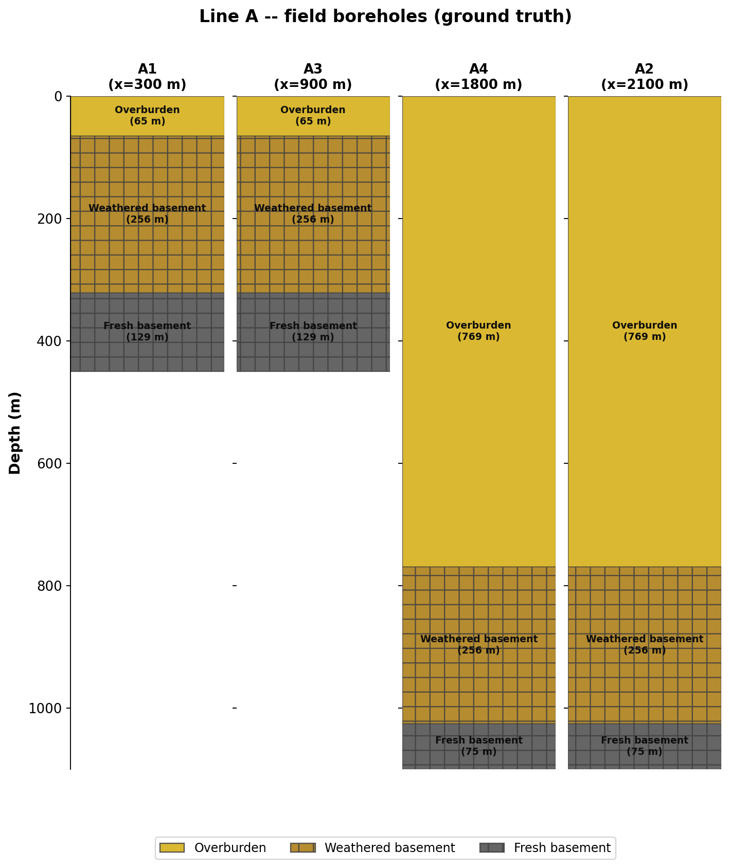
Line A’s four boreholes, ordered by x. A1/A3 (footwall)
only needed 450 m to confirm fresh basement; A4/A2
(downthrown) needed 1100 m for the same confirmation – the fault
throw, read directly off real drilling depths rather than off a
model. The blank space below A1/A3 is left genuinely blank,
with no panel border drawn into it: nothing was drilled there, so
there is nothing to frame.#
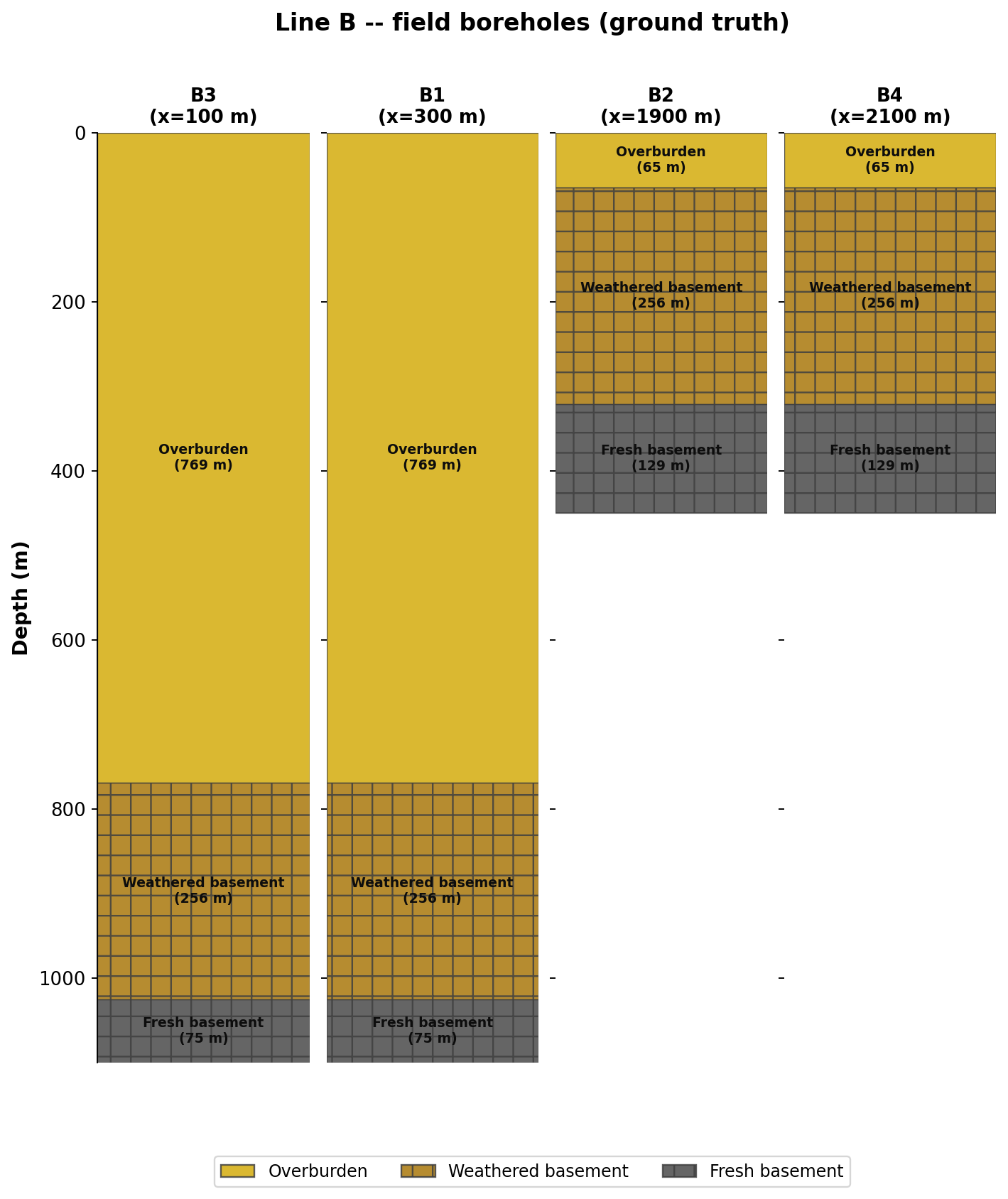
Line B’s four boreholes, ordered by x. The pattern mirrors Line A
with the sides swapped – downthrown_side="left" here, so the
deep contact sits under B3/B1 instead.#
18.21.4. Calibrate against the two boreholes#
ModelCalibrator blends borehole evidence into
the raw calculated model (CRM): cells within ptol (10% here) of a
nearby borehole’s true resistivity are replaced outright; everything
else is classified from the regional table alone. Stations farther than
max_borehole_distance (500 m, the default) from any borehole get no
direct TRES influence at all:
>>> from pathlib import Path
>>> from pycsamt.interp import ResistivityModel, ModelCalibrator
>>> from pycsamt.models.occam2d import InversionResult

>>> result_a = InversionResult(Path("runs/line_a_occam2d"))
>>> model_a = ResistivityModel.from_occam2d(result_a).clip_to_stations()
>>> cal_a = ModelCalibrator(ptol=0.10, db=regional_db, verbose=False)
>>> _ = cal_a.fit(model_a, [bh_a1, bh_a2])
>>> nm_a = cal_a.calibrated_model()
>>> nm_a.method
'occam2d+calibrated'
A1 is 600 m from station L09 (x=900 m) and A2 is 300 m from
L18 (x=1800 m) – both within reach in principle, though whether TRES
replacement actually fires at a given station depends on whether the
raw CRM resistivity there ever comes close enough to the borehole’s true
value, which the validation section below shows is not guaranteed just
because a borehole is nearby.
18.21.5. See where calibration actually changed the model#
cal_a.misfit_map() gives a per-column G (%) figure quantifying how
much a station’s calibrated column differs from the raw CRM:
>>> mm_a = cal_a.misfit_map()
>>> mm_a.shape
(32, 50)
>>> round(float(mm_a.min()), 2), round(float(mm_a.max()), 2)
(8.46, 12.24)
Every one of Line A’s 50 columns sits at 8-12% misfit – not just the
two calibrated ones. That is real, and it is not a sign that something
went wrong: fit() runs
classify()-based autolayer
reclassification on every column outside max_borehole_distance of
a borehole, not just a straight TRES swap near the two that are close
enough. Autolayering alone – collapsing a smooth, continuous CRM
column into a handful of discrete rock-database bins – already moves
most cells’ resistivity by a similar margin everywhere it runs, so the
misfit floor sits well above zero across the whole line, not only away
from the boreholes.
Occam2D’s own mesh reaches almost 10 km depth for numerical-boundary
reasons that have nothing to do with the shallow geology this survey
cares about; plotted at full depth, the interesting top 1600 m would be
squeezed into a sliver of the figure. The figures below crop that
directly with depth_max (shown next); the same crop is available
without any topography draping through the new
clip_to_depth(), useful whenever
a plain flat-depth model is all that is needed:
>>> model_a.n_z, model_a.clip_to_depth(1600.0).n_z
(32, 19)
Rather than the flat, no-terrain PlotCalibratedModel
panel, the figure below drapes CRM, NM, and the misfit map over this
line’s real terrain with plot_topo_section() – the
same function Build A Two-Line Occam2D Survey For Interpretation used for the
topography figure in Part 1 – plus the shared inversion station
marker (a black-edged, white-filled downward triangle) and every
station’s real elevation, resolvable directly from a
ResistivityModel since CRM and NM both are
one. The misfit array is not a resistivity grid, so it goes through the
generic plot_topo_array() instead, which drapes and
colour-maps any 2-D field without assuming a log10(rho) transform.
Both functions accept depth_max directly, cropping out Occam2D’s
own numerical-boundary mesh (it reaches almost 10 km depth for reasons
that have nothing to do with this survey’s shallow geology) down to the
top 1600 m that is actually worth looking at. Because the misfit floor
sits at 8-12% almost everywhere rather than the more typical case of a
mostly-untouched line, the colour scale is widened to vmax=15
rather than the tighter 0-10% range that would suit that typical case:
View the calibration-effect figure source codeClick to inspect and copy the complete code
 1def make_calibration_effect_figures():
 2    """CRM vs calibrated NM vs the G (%) misfit map, draped over real
 3    topography with the shared inversion station marker, for both
 4    lines -- the direct visual record of where ModelCalibrator's
 5    soft-replace step actually changed the raw inversion, and by how
 6    much.
 7
 8    All three panels are clipped to the top 1600 m -- Occam2D's own
 9    mesh reaches almost 10 km depth for numerical-boundary reasons,
10    which would otherwise squeeze the entire zone of geological
11    interest into a sliver of the figure. CRM/NM use
12    pycsamt.topo.plot_topo_section directly (they are real
13    ResistivityModel objects); the misfit map is not a resistivity
14    grid, so it uses the generic pycsamt.topo.plot_topo_array instead.
15    misfit_map()'s per-column G (%) runs 6-13% almost everywhere on
16    this survey (autolayer reclassification touches every column
17    outside max_borehole_distance of a borehole, not just the
18    calibrated ones), so vmax=15 is used instead of the 0-10% range
19    that would suit a typical, mostly-untouched line.
20
21    CRM and NM share one colour scale, so they share one colorbar
22    rather than two identical ones. The three panels are laid out on a
23    GridSpec with a dedicated, fixed-width colorbar column instead of
24    letting each plotting call attach its own -- plot_topo_section's
25    colorbar (mpl_toolkits' make_axes_locatable, a fixed percentage of
26    its own axes) and a bare fig.colorbar (matplotlib's default
27    fraction/pad) do not reserve the same width, which otherwise leaves
28    the misfit panel a different width from CRM/NM.
29    """
30    for line, calib_spec, valid_spec, workdir in (
31        (LINE_A, LINE_A_CALIB_BOREHOLES, LINE_A_VALID_BOREHOLES, "line_a_occam2d"),
32        (LINE_B, LINE_B_CALIB_BOREHOLES, LINE_B_VALID_BOREHOLES, "line_b_occam2d"),
33    ):
34        calib, _ = build_boreholes(line, calib_spec, valid_spec)
35        model, cal = load_calibrated_model(workdir, calib)
36        nm = cal.calibrated_model()
37        mm = cal.misfit_map()
38        elev = elevation_for_line(line, model.station_x)
39
40        fig = plt.figure(figsize=(12, 12))
41        gs = fig.add_gridspec(
42            3, 2, width_ratios=[30, 1], height_ratios=[1, 1, 1.08],
43            hspace=0.65, wspace=0.06,
44        )
45        ax_crm = fig.add_subplot(gs[0, 0])
46        ax_nm = fig.add_subplot(gs[1, 0], sharex=ax_crm)
47        ax_g = fig.add_subplot(gs[2, 0], sharex=ax_crm)
48        cax_rho = fig.add_subplot(gs[0:2, 1])
49        cax_g = fig.add_subplot(gs[2, 1])
50
51        common = dict(
52            elevation=elev, station_x=model.station_x,
53            station_names=model.station_names, depth_max=1600.0,
54        )
55        plot_topo_section(
56            model, ax=ax_crm, cmap="jet", vmin=1.0, vmax=5.0,
57            colorbar=False, title="CRM -- inversion result", **common,
58        )
59        plot_topo_section(
60            nm, ax=ax_nm, cmap="jet", vmin=1.0, vmax=5.0,
61            colorbar=False, title="NM -- calibrated model", **common,
62        )
63        plot_topo_array(
64            model.x_centers, model.z_centers, mm, ax=ax_g,
65            cmap="RdYlBu_r", vmin=0.0, vmax=15.0, colorbar=False,
66            title="Misfit G (%)", **common,
67        )
68        fig.colorbar(
69            ax_crm.collections[0], cax=cax_rho,
70            label=r"$\log_{10}\rho$ ($\Omega\cdot$m)",
71        )
72        fig.colorbar(ax_g.collections[0], cax=cax_g, label="G (%)")
73
74        # Only the bottom panel needs the shared x-axis label/ticks --
75        # repeating "Profile distance (km)" on all three, this close
76        # together, just crowds the titles above each lower panel.
77        ax_crm.set_xlabel("")
78        ax_nm.set_xlabel("")
79        ax_crm.tick_params(labelbottom=False)
80        ax_nm.tick_params(labelbottom=False)
81
82        fig.suptitle(
83            f"{line['label']} -- CRM vs calibrated NM, real topography (top 1600 m)",
84            fontweight="bold", y=0.995,
85        )
86        letter = line["label"].split()[-1].lower()
87        fig.savefig(IMAGES / f"calibration_effect_{letter}.png", dpi=170, bbox_inches="tight")
88        plt.close(fig)
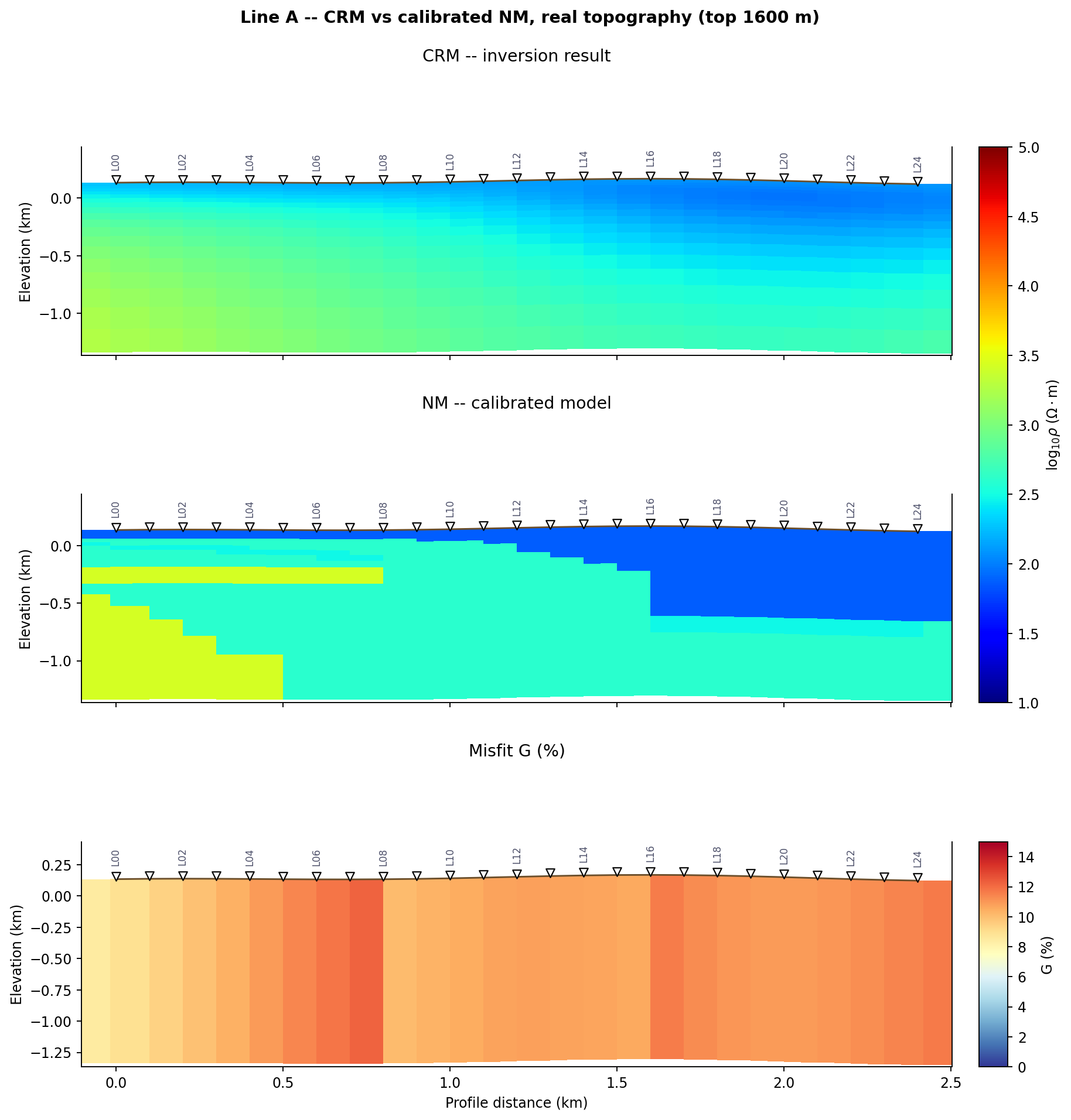
Line A, draped over its real terrain (the ridge peaking near
L14-L18). The misfit panel is lowest (pale yellow, near
8%) right at L00/L24 where the calibration boreholes sit,
and highest (orange, near 12%) at the columns farthest from both –
exactly the gradient autolayer-dominated misfit should produce.#
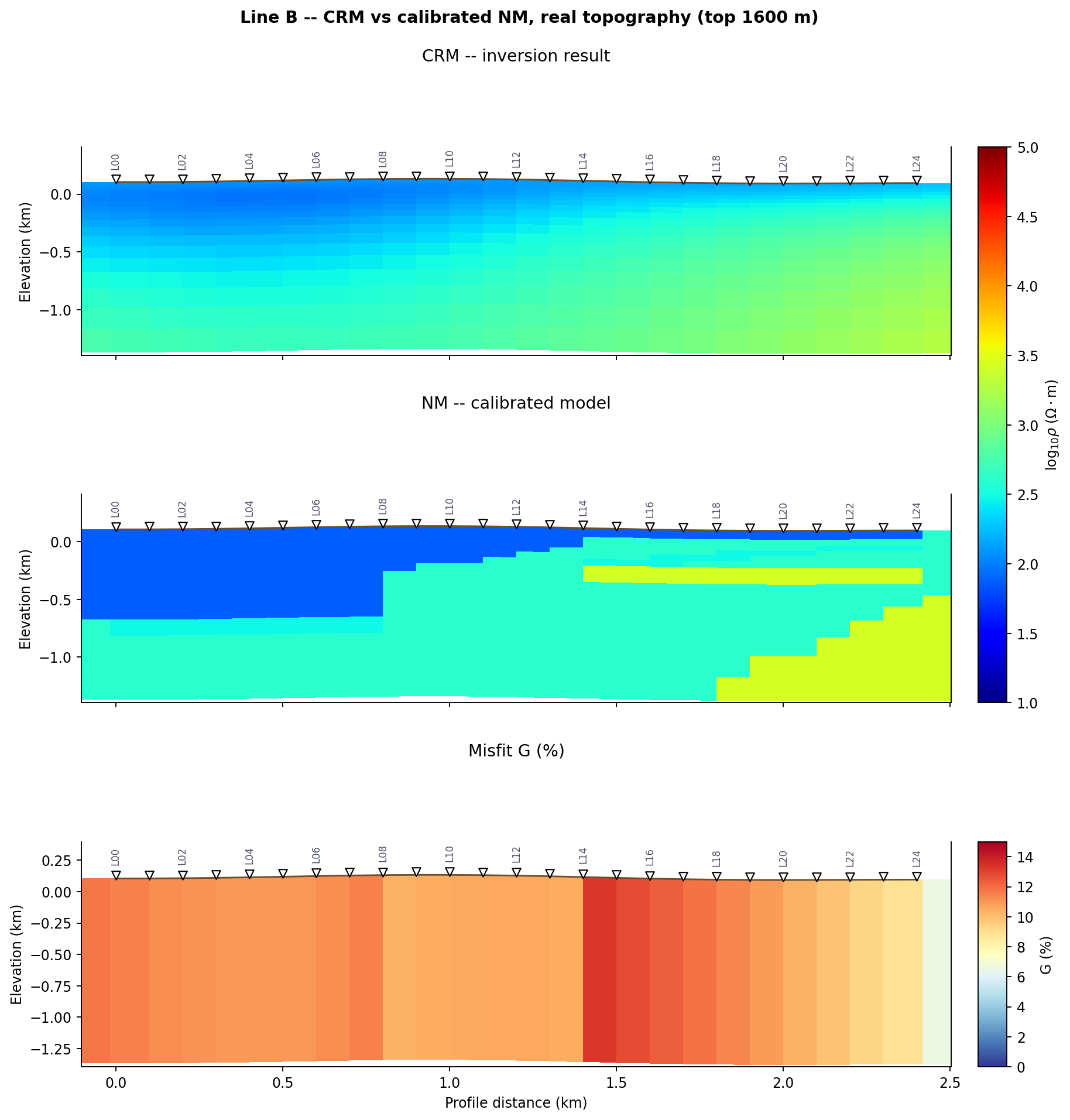
Line B shows the same pattern with its own boreholes and its own
(independent) terrain: misfit peaks (dark red, above 13%) roughly
midway between B1 (x=300 m) and B2 (x=1900 m) – the point
on the line farthest from either calibration borehole – and falls
toward both ends.#
18.21.6. Classify into lithology and draw the fence diagram#
cal_a.stratigraphic_logs() classifies every station’s calibrated
column into merged lithology layers with the regional table, the same
mechanism Lithology classification covers in depth:
>>> logs_a = cal_a.stratigraphic_logs()
>>> len(logs_a)
25
>>> log_l00 = [log for log in logs_a if log.station_name == "L00"][0]
>>> [(round(l.top, 1), round(l.bottom, 1), l.lithology) for l in log_l00.layers]
[(0.0, 76.9, 'Overburden'), (74.9, 322.1, 'Weathered basement'), (317.2, 465.8, 'Fresh basement'), (459.2, 659.2, 'Weathered basement'), (650.3, 10684.7, 'Fresh basement')]
Station L00 sits directly at A1’s own position, and the shallow
boundary (overburden ending around 77 m, against a true 65 m) is close
– but the layer sequence oscillates once, back to “Weathered basement”
around 460-660 m before returning to “Fresh basement”, rather than
settling cleanly. That is genuine classification noise, not a display
bug: the soft-replace step only pulls individual cells toward the true
value within ptol; it does not smooth the resulting sequence
afterward, so a column that dips in and out of the 10% tolerance band
near the true transition depth can flicker between two lithologies for
a few cells before committing to one.
The fence diagram below renders every one of Line A’s 25 classified
logs side by side, so that flicker – and the overall footwall-to-
downthrown transition – is visible across the whole profile at once.
PlotFenceDiagram takes an elevation_m
array (one value per log, same order) and draws a real terrain strip
above the panels, with the same shared inversion station marker
used everywhere else on this page:
View the fence-diagram figure source codeClick to inspect and copy the complete code
 1def make_fence_diagrams():
 2    """Classified fence diagram for every station, with a real terrain
 3    strip and the shared ``inversion`` station marker drawn above the
 4    panels -- the same station-index convention
 5    pycsamt.topo.draw_topo_strip uses for pseudosections, applied here
 6    via PlotFenceDiagram's own elevation_m parameter."""
 7    for line, calib_spec, valid_spec, workdir in (
 8        (LINE_A, LINE_A_CALIB_BOREHOLES, LINE_A_VALID_BOREHOLES, "line_a_occam2d"),
 9        (LINE_B, LINE_B_CALIB_BOREHOLES, LINE_B_VALID_BOREHOLES, "line_b_occam2d"),
10    ):
11        calib, _ = build_boreholes(line, calib_spec, valid_spec)
12        model, cal = load_calibrated_model(workdir, calib)
13        logs = cal.stratigraphic_logs()
14        elev = elevation_for_line(line, model.station_x)
15        fig = iplot.PlotFenceDiagram(
16            logs, max_depth=1600.0, elevation_m=elev,
17            title=f"{line['label']} -- classified fence diagram",
18        ).plot()
19        fig.savefig(IMAGES / f"fence_{line['label'].split()[-1].lower()}.png", dpi=170, bbox_inches="tight")
20        plt.close(fig)
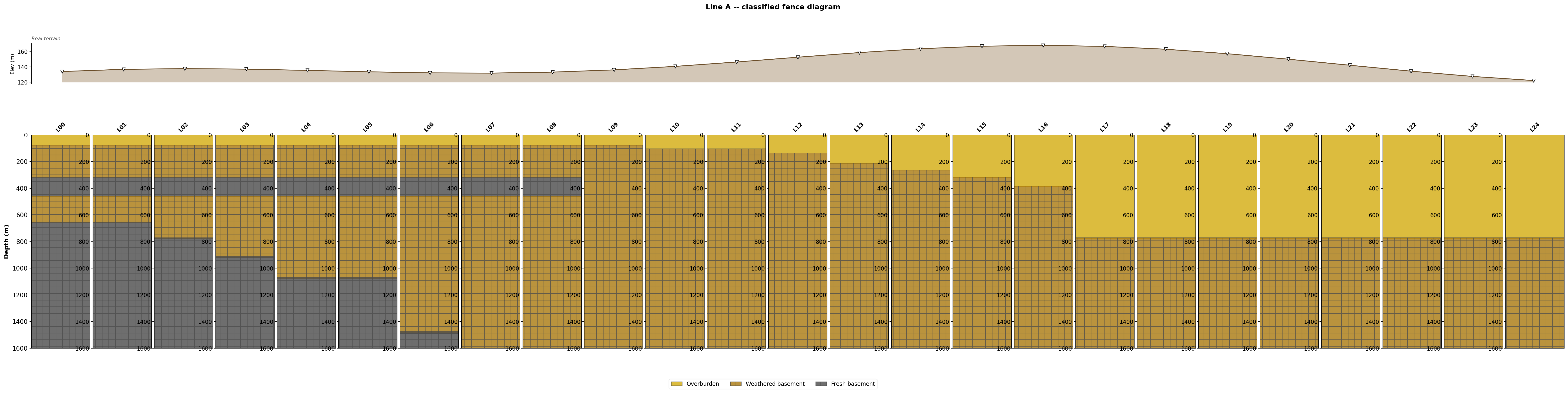
PlotFenceDiagram for Line A, all 25
stations, with its real terrain strip on top. Grey (fresh basement)
sits shallow through roughly L00-L06 – the footwall, close
to A1 – then the boundary steps down through the fault-crossing
zone before the profile settles into the deeper, downthrown pattern
from about L17 onward, close to A2. Note that the strip uses
station index along the x-axis to line up with the equal-width
panels below, not real chainage.#
18.21.7. Record the fault as structural evidence#
Nothing in the classified section above places the fault – the
lithology boundary just described is a smoothed reflection of it, not a
located pick. FaultTrace records the fault
directly, from what is actually known about it here (the same true
geometry Build A Two-Line Occam2D Survey For Interpretation used to build the earth
model in the first place, standing in for what a real project would
learn from surface mapping, a resistivity offset, or a nearby drill
result):
>>> from pycsamt.geology import FaultTrace
>>> fault_a = FaultTrace(
...     x=1200.0, dip_deg=65.0, downthrown_side="right", throw_m=700.0,
...     sense="normal", evidence="true model (synthetic control)",
... )
>>> fault_a
FaultTrace(x=1200.0 m, dip=65 deg, down=right, throw=700.0 m)
Line B’s own fault trace is identical in kind, built from its own
geometry (x=1400.0, dip_deg=47.0, downthrown_side="left") –
the same true fault system Part 1 introduced, crossed at a shallower
apparent dip. Drawing both lines’ calibrated sections with the true
fault trace and all four boreholes overlaid makes the relationship
between them concrete – and doing it over real terrain, the way the
calibration-effect figures above already do, means the fault trace and
every borehole need converting from flat (x, depth) into
terrain-following (x, elevation) first. interp_elev()
(the same function this page already relies on for every terrain
lookup) gives the local elevation at any along-profile x; the fault
trace’s own x = fault_x + z / tan(apparent_dip) relationship then
becomes elevation = interp_elev(x) - z at each depth sample, and
each borehole’s line runs from interp_elev(bh.x) down to
interp_elev(bh.x) - bh.max_depth:
View the structural-overlay figure source codeClick to inspect and copy the complete code
 1def make_structural_section_figure():
 2    """Draw both lines' calibrated sections draped over real topography,
 3    with the true fault trace and every borehole overlaid in the same
 4    terrain-following (elevation, not flat depth) coordinates the
 5    background section itself uses.
 6
 7    pycsamt.topo.plot_topo_section does the draping and draws the
 8    station markers/labels; the fault trace and borehole traces are
 9    plotted afterwards on the same axes, converted from
10    (x, depth)-space into (x, elevation)-space with the same
11    pycsamt.topo.interp_elev this page's boreholes are built against.
12    """
13    fig, axes = plt.subplots(2, 1, figsize=(11, 10))
14    specs = (
15        (LINE_A, LINE_A_CALIB_BOREHOLES, LINE_A_VALID_BOREHOLES, "line_a_occam2d"),
16        (LINE_B, LINE_B_CALIB_BOREHOLES, LINE_B_VALID_BOREHOLES, "line_b_occam2d"),
17    )
18    for ax, (line, calib_spec, valid_spec, workdir) in zip(axes, specs):
19        calib, valid = build_boreholes(line, calib_spec, valid_spec)
20        model, cal = load_calibrated_model(workdir, calib)
21        nm = cal.calibrated_model()
22        elev = elevation_for_line(line, model.station_x)
23        chain_km = model.station_x / 1000.0
24        elev_km = elev / 1000.0
25
26        plot_topo_section(
27            nm, ax=ax, elevation=elev, station_x=model.station_x,
28            station_names=model.station_names, depth_max=1600.0,
29            cmap="turbo_r", vmin=1.5, vmax=4.0,
30            title=f"{line['label']} -- calibrated model, true fault, and boreholes",
31        )
32
33        def elev_at_km(x_m):
34            return float(interp_elev(chain_km, elev_km, np.array([x_m / 1000.0]))[0])
35
36        fault = fault_trace_for_line(line)
37        z = np.linspace(0.0, 1600.0, 60)
38        direction = 1.0 if fault.downthrown_side == "right" else -1.0
39        x_line_m = fault.x + direction * z / np.tan(np.deg2rad(fault.dip_deg))
40        y_line_km = np.array(
41            [elev_at_km(xi) - zi / 1000.0 for xi, zi in zip(x_line_m, z)]
42        )
43        ax.plot(x_line_m / 1000.0, y_line_km, color="white", linewidth=2.5,
44                linestyle="--", zorder=6,
45                label=f"true fault ({fault.dip_deg:.0f} deg apparent dip)")
46
47        for bh, bold, ls, lw in (
48            *((bh, True, "-", 2.0) for bh in calib),
49            *((bh, False, ":", 1.2) for bh in valid),
50        ):
51            e0_km = elev_at_km(bh.x)
52            y_top_km = e0_km
53            y_bot_km = e0_km - bh.max_depth / 1000.0
54            ax.plot([bh.x / 1000.0, bh.x / 1000.0], [y_top_km, y_bot_km],
55                    color="black", linewidth=lw, linestyle=ls, zorder=6)
56            ax.text(bh.x / 1000.0, y_bot_km - 0.03, bh.name, ha="center",
57                    va="top", fontsize=8, fontweight="bold" if bold else None,
58                    style=None if bold else "italic", zorder=7)
59
60        ax.legend(loc="lower right", fontsize=8)
61    fig.tight_layout()
62    fig.savefig(IMAGES / "structural_overlay.png", dpi=170, bbox_inches="tight")
63    plt.close(fig)
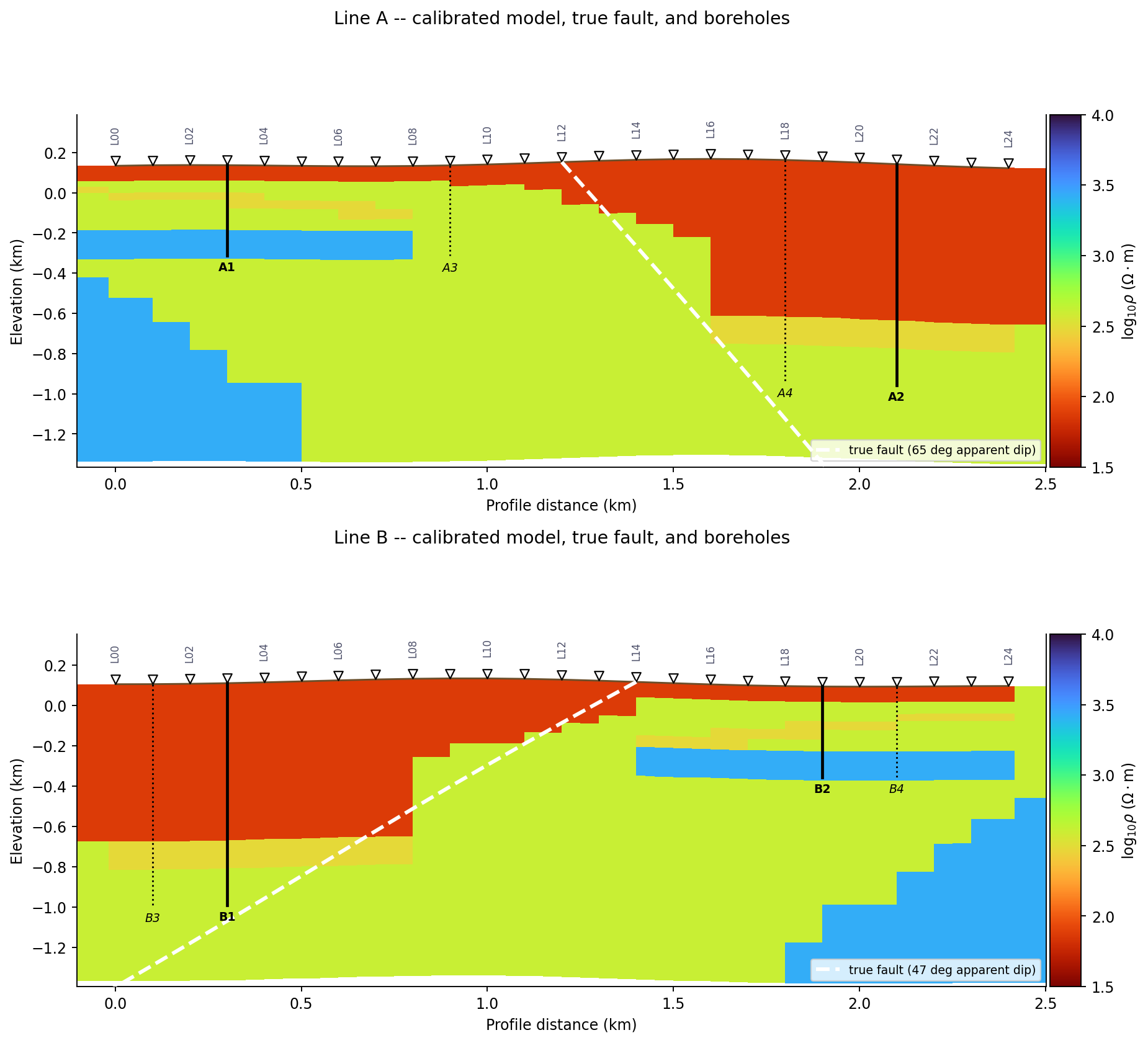
Both lines draped over their own real terrain, with the inversion
station marker and L00-L24 labels from
plot_topo_section() along the top. Solid lines
and bold labels are calibration boreholes (A1/A2,
B1/B2); dotted lines and italic labels are the held-out
validation boreholes – both now hanging from the real terrain
surface rather than a flat datum. The sharp, blocky colouring
immediately around each calibration borehole is the soft-replace
step visibly overriding the smooth Occam2D image with real TRES
values; everywhere else keeps the raw inversion’s own smooth
gradient.#
18.21.8. Validate against the held-out boreholes#
This is the step that actually tests whether calibration and
classification recovered something real, rather than just producing a
plausible-looking picture. A3 and A4 were never shown to the
calibrator:
>>> bh_a3 = borehole_from_true(grid_a, "A3", 900.0, 450.0)
>>> bh_a4 = borehole_from_true(grid_a, "A4", 1800.0, 1100.0)
>>> logs_by_station = {log.station_name: log for log in logs_a}

>>> log_l09 = logs_by_station["L09"]  # nearest station to A3 (exact: same x)
>>> bh_a3.intervals[0].bottom, log_l09.layers[0].bottom   # overburden base, true vs classified
(65.0, 76.93395000000001)
>>> bh_a3.intervals[-1].top    # true basement top
321.0
>>> next(l.top for l in log_l09.layers if l.lithology == "Fresh basement")
2345.512975
The shallow overburden boundary is close either way (77 m classified
against 65 m true) – resolvable because Occam2D’s own shallow
resolution is good almost everywhere on this line, calibration borehole
nearby or not. The basement top is not close at all: 2346 m classified
against 321 m true, off by a factor of more than seven. A4
(downthrown, 300 m from calibration borehole A2, well inside
max_borehole_distance) does not fare better:
>>> log_l18 = logs_by_station["L18"]  # nearest station to A4 (exact: same x)
>>> bh_a4.intervals[0].bottom, log_l18.layers[0].bottom
(769.0, 779.6850000000001)
>>> bh_a4.intervals[-1].top
1025.0
>>> next(l.top for l in log_l18.layers if l.lithology == "Fresh basement")
5849.26135
Proximity to a calibration borehole did not save this one either. The
reason is visible directly in the section figure above: the raw
Occam2D image on the downthrown side never actually recovers a
resistivity anywhere close to 3000 Ω·m at any depth this model
resolves, so the soft-replace step – which only fires within ptol
of the true value – never has a matching cell to grab onto near the
true basement depth, calibration borehole nearby or not. Depth of
investigation, not distance to the nearest borehole, is the binding
constraint here.
Line B’s footwall validation borehole, B4 (x=2100 m, 300 m from
calibration borehole B2), tells the opposite story – because on
Line B’s footwall side the true basement sits shallow (321 m, the
same depth A1/A3 see on Line A), well within what this model
actually resolves:
>>> grid_b = Grid2D.layered_with_fault(
...     true_layers, fault_x_m=1400.0, apparent_dip_deg=47.0,
...     throw_m=700.0, downthrown_side="left",
...     nx=60, nz=50, x_max=2400.0, z_max=1600.0, n_stations=25, name="Line B",
... )
>>> bh_b4 = borehole_from_true(grid_b, "B4", 2100.0, 450.0)
>>> bh_b4.intervals[-1].top
321.0

>>> result_b = InversionResult(Path("runs/line_b_occam2d"))
>>> model_b = ResistivityModel.from_occam2d(result_b).clip_to_stations()
>>> bh_b1 = borehole_from_true(grid_b, "B1", 300.0, 1100.0)
>>> bh_b2 = borehole_from_true(grid_b, "B2", 1900.0, 450.0)
>>> cal_b = ModelCalibrator(ptol=0.10, db=regional_db, verbose=False)
>>> _ = cal_b.fit(model_b, [bh_b1, bh_b2])
>>> logs_b = {log.station_name: log for log in cal_b.stratigraphic_logs()}
>>> log_l21 = logs_b["L21"]  # nearest station to B4
>>> next(l.top for l in log_l21.layers if l.lithology == "Fresh basement")
317.175025
317 m classified against 321 m true – within 4 m, the best match on
either line. Four validation boreholes, two clear outcomes: the shallow
overburden contact classifies well everywhere on both lines regardless
of calibration proximity; the basement contact classifies well only
where it is shallow enough for Occam2D to have actually resolved it, and
badly wherever it is not, independent of how close a calibration
borehole happens to sit. Reporting both, rather than only the flattering
B4 result, is the entire point of holding boreholes out in the first
place.
18.21.9. What this adds up to#
The raw inversion result from Build A Two-Line Occam2D Survey For Interpretation
showed a smooth resistivity gradient and nothing else – no fault, no
named lithology, no way to tell a well-resolved boundary from a poorly
resolved one. Everything on this page came from combining that result
with independent evidence: RockDatabase turned
resistivity into lithology names a project actually recognises;
ModelCalibrator pulled the model toward real
measurements near the two calibration boreholes, and its misfit_map
showed exactly how far that influence actually reaches;
FaultTrace placed the fault using what is
actually known about it, rather than reading a position off a smoothed
image that was never going to show one; and the two held-out boreholes
turned “this looks reasonable” into an honest, checkable claim about
where the result can and cannot be trusted. The borehole fence,
calibration-effect, classified fence, and structural-overlay figures
along the way are all built the same way: real
pycsamt.interp.plot classes and, wherever real terrain and
station markers belong in the picture, real pycsamt.topo
functions – called directly on this page’s own real objects, never a
hand-drawn illustration.
18.21.10. See Also#
- Build A Two-Line Occam2D Survey For Interpretation
Builds the two real Occam2D lines this page interprets.
- Interpretation workflow
The general calibrate-classify-review sequence this page follows, on a smaller synthetic fixture.
- Rock resistivity database
Why a project-specific rock table changes the classified answer even when the resistivity does not.
- Borehole logs
Borehole/Intervalmechanics used throughout this page.- Structural measurements
FaultTrace’s apparent-dip geometry, covered in full.- Uncertainty and validation
Where to go next for a quantitative, sampled treatment of the same kind of uncertainty this page’s validation section found by hand.