
8.3. Petrophysical toolkit#
Hydrogeophysical interpretation and Uncertainty and validation call
ArchieModel,
WaxmanSmitsModel, and a handful of
derived quantities as internal steps inside
EMHydroModel and
MonteCarloHydro. This page treats
pycsamt.interp.petrophysics as a toolkit in its own right: every
constitutive model and standalone conversion it exposes, called directly
rather than through those higher-level wrappers, so each piece can be
reasoned about independently before trusting it inside a larger workflow.
Where Lithology classification answers which rock is this cell,
pycsamt.interp.petrophysics answers how much water does this
resistivity imply, and how confidently – a quantitative question that
needs a constitutive model (Archie or Waxman-Smits), an admissibility check
(Hashin-Shtrikman), and explicit pore-water and grain-size assumptions, not
just a lookup table.
>>> from pycsamt.interp.petrophysics import ArchieModel

>>> archie = ArchieModel(m=1.8, n=2.0, a=1.0)
>>> archie
ArchieModel(m=1.8, n=2.0, a=1.0)
8.3.1. Archie’s law#
Archie’s law (1942) relates formation resistivity to porosity and water saturation through the formation factor \(F = a\,\phi^{-m}\) and
ArchieModel implements the forward direction and three independent
inverses – saturation, porosity, fluid_resistivity – each
solving the same equation for a different unknown given the other two.
Using rho_w=20 \(\Omega\mathrm{m}\) (typical fresh groundwater, the
same value used throughout Hydrogeophysical interpretation):
>>> round(archie.formation_factor(0.28), 3)
9.888
>>> round(archie.forward(phi=0.28, Sw=1.0, rho_w=20.0), 1)
197.8
>>> round(archie.forward(phi=0.28, Sw=0.6, rho_w=20.0), 1)
549.3
Saturated (\(S_w=1\)) rock is markedly more conductive than the same rock at 60% saturation – lower water content means fewer conductive ion paths, so resistivity rises as \(S_w^{-n}\) even though porosity and pore-water chemistry are unchanged. The three inverses recover any one input from the other two and the measured resistivity:
>>> round(archie.saturation(rho=250.0, phi=0.28, rho_w=20.0), 3)
0.889
>>> round(archie.porosity(rho=250.0, Sw=1.0, rho_w=20.0), 3)
0.246
>>> round(archie.fluid_resistivity(rho=250.0, phi=0.28, Sw=1.0), 2)
25.28
>>> round(archie.water_content(phi=0.28, Sw=0.6), 3)
0.168
water_content is the simple product \(\theta=\phi\,S_w\) – the
volumetric fraction of the rock that is actually water, as opposed to
\(S_w\) alone, which only says what fraction of the pore space is
water and says nothing if porosity itself is small.
The cementation exponent m and saturation exponent n play different roles: m sets how strongly resistivity depends on porosity (it appears only in the formation factor), and n sets how strongly it depends on saturation (it appears only in the \(S_w^{-n}\) term). Sweeping each independently makes that split visible:
>>> import numpy as np
>>> import matplotlib.pyplot as plt

>>> phi_grid = np.linspace(0.05, 0.45, 100)
>>> Sw_grid = np.linspace(0.05, 1.0, 100)

>>> fig, (ax1, ax2) = plt.subplots(1, 2, figsize=(10, 4.5))
>>> for m in (1.3, 1.8, 2.3):
...     a_m = ArchieModel(m=m, n=2.0, a=1.0)
...     rho_m = a_m.forward(phi=phi_grid, Sw=1.0, rho_w=20.0)
...     _ = ax1.plot(phi_grid, rho_m, label=f"m={m}")
>>> _ = ax1.set_yscale("log")
>>> _ = ax1.set_xlabel(r"$\phi$")
>>> _ = ax1.set_ylabel(r"$\rho$ ($\Omega\,\mathrm{m}$)")
>>> _ = ax1.set_title(r"Cementation exponent $m$ ($S_w=1.0$)")
>>> _ = ax1.legend(fontsize=8)
>>> _ = ax1.grid(alpha=0.3)

>>> for n in (1.8, 2.0, 2.5):
...     a_n = ArchieModel(m=1.8, n=n, a=1.0)
...     rho_n = a_n.forward(phi=0.28, Sw=Sw_grid, rho_w=20.0)
...     _ = ax2.plot(Sw_grid, rho_n, label=f"n={n}")
>>> _ = ax2.set_yscale("log")
>>> _ = ax2.set_xlabel(r"$S_w$")
>>> _ = ax2.set_ylabel(r"$\rho$ ($\Omega\,\mathrm{m}$)")
>>> _ = ax2.set_title(r"Saturation exponent $n$ ($\phi=0.28$)")
>>> _ = ax2.legend(fontsize=8)
>>> _ = ax2.grid(alpha=0.3)
>>> fig.tight_layout()
>>> fig.savefig("review/archie_sensitivity.png", dpi=200, bbox_inches="tight")
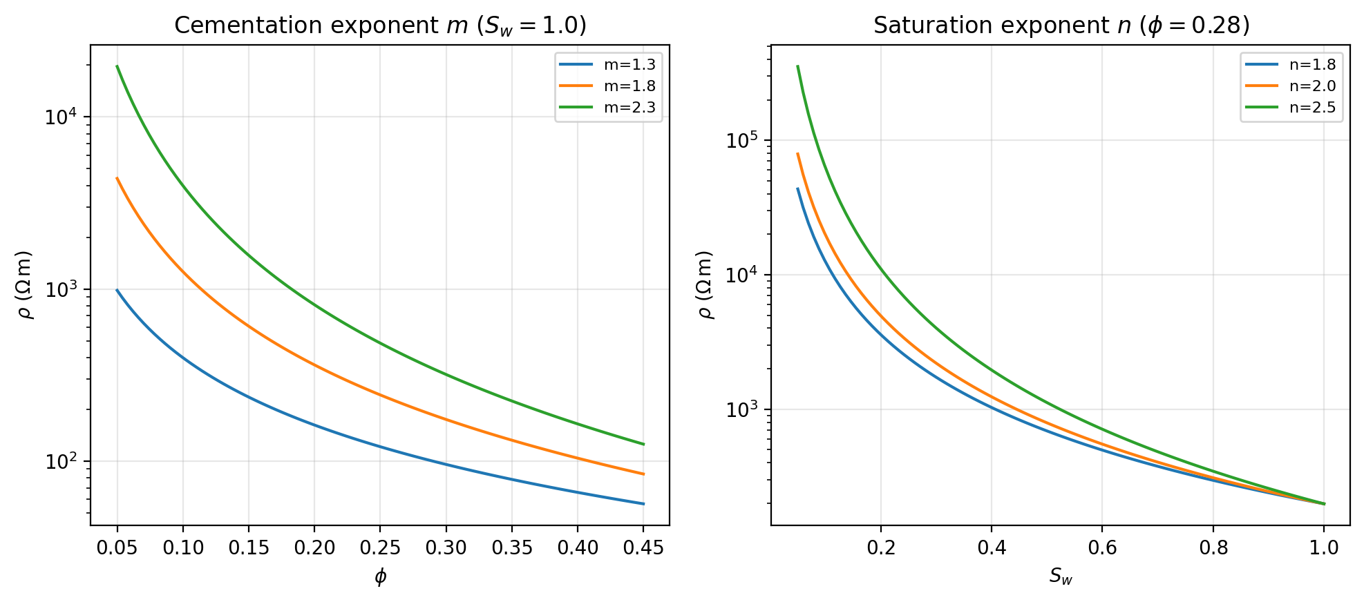
Left: varying m at full saturation shifts the whole \(\rho\)-vs- \(\phi\) curve, since \(S_w=1\) makes the \(S_w^{-n}\) term drop out entirely – n has no effect here, which is why all three panels would overlap if plotted against n instead. Right: varying n at fixed porosity shows the opposite – the curves converge exactly at \(S_w=1\) (where \(S_w^{-n}=1\) regardless of n) and diverge as saturation drops, most steeply for the largest n.#
Warning
ArchieModel silently clips every input and output to a safety range
(\(\phi\in[10^{-4}, 0.99]\), \(S_w\in[10^{-4}, 1]\),
\(\rho\in[10^{-2}, 10^{7}]\ \Omega\mathrm{m}\)) rather than raising.
A porosity of exactly 0 or a resistivity outside that range will return
a clipped, physically-questionable value instead of an error – check
inputs against these ranges yourself before trusting an inversion at
the edges of a real dataset.
8.3.2. Effect of clay conductivity#
Clay minerals add an extra, saturation-independent conduction path along
their charged surfaces. Archie’s law has no term for it, so
applying Archie to a clay-bearing formation systematically overestimates
resistivity for a given \(\phi\) and \(S_w\) – which, read
backwards through the inverse, means it underestimates saturation. The
Waxman-Smits model,
WaxmanSmitsModel, adds that term
explicitly:
>>> from pycsamt.interp.petrophysics import WaxmanSmitsModel

>>> ws0 = WaxmanSmitsModel(m=1.8, n=2.0, a=1.0, sigma_s=0.0)
>>> round(ws0.forward(phi=0.28, Sw=0.6, sigma_w=50.0), 1)
549.3
>>> round(archie.forward(phi=0.28, Sw=0.6, rho_w=20.0), 1)
549.3
With sigma_s=0 the two models agree exactly – sigma_w is pore-water
conductivity in mS/m, and 50 mS/m converts to the same
\(\rho_w=1/(0.05\ \mathrm{S/m})=20\ \Omega\mathrm{m}\) used above, so
Waxman-Smits is Archie’s law with the clay term switched off. Turning
sigma_s on pulls resistivity down at every saturation, most visibly at
low \(S_w\) where the formation’s own conductivity is smallest relative
to the fixed clay contribution:
>>> ws_clay = WaxmanSmitsModel(m=1.8, n=2.0, a=1.0, sigma_s=0.01)
>>> round(ws_clay.forward(phi=0.28, Sw=0.6, sigma_w=50.0), 1)
412.0

>>> fig, ax = plt.subplots(figsize=(6.5, 4.5))
>>> for sigma_s in (0.0, 0.01, 0.05):
...     ws_i = WaxmanSmitsModel(m=1.8, n=2.0, a=1.0, sigma_s=sigma_s)
...     rho_i = ws_i.forward(phi=0.28, Sw=Sw_grid, sigma_w=50.0)
...     label = "Archie (clay-free)" if sigma_s == 0.0 else f"$\\sigma_s$={sigma_s} S/m"
...     _ = ax.plot(Sw_grid, rho_i, label=label)
>>> _ = ax.set_yscale("log")
>>> _ = ax.set_xlabel(r"$S_w$")
>>> _ = ax.set_ylabel(r"$\rho$ ($\Omega\,\mathrm{m}$)")
>>> _ = ax.set_title(r"Waxman-Smits at $\phi=0.28$, $\sigma_w=50$ mS/m")
>>> _ = ax.legend(fontsize=9)
>>> _ = ax.grid(alpha=0.3)
>>> fig.tight_layout()
>>> fig.savefig("review/waxman_smits_clay.png", dpi=200, bbox_inches="tight")
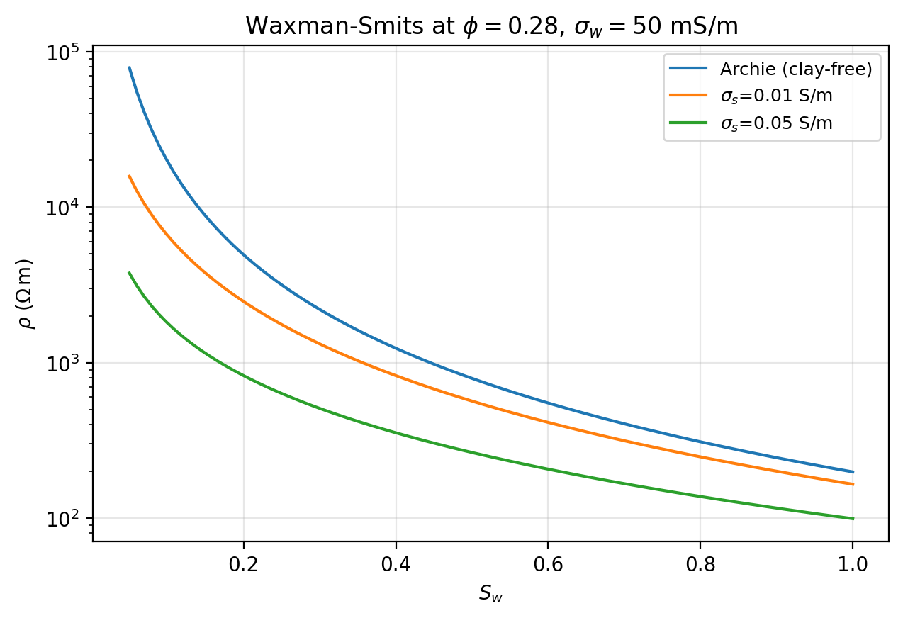
Higher sigma_s pulls every curve down without changing its shape.
At \(S_w=1\) the gap between clay-free and \(\sigma_s=0.05\)
S/m is still roughly a factor of five – clay conduction does not
disappear just because the rock is fully saturated.#
Inverting Waxman-Smits for saturation has no closed form, so
WaxmanSmitsModel.saturation root-finds it numerically with
scipy.optimize.brentq() per cell:
>>> rho_obs = ws_clay.forward(phi=0.28, Sw=0.6, sigma_w=50.0)
>>> round(ws_clay.saturation(rho=rho_obs, phi=0.28, sigma_w=50.0), 3)
0.6
Warning
The root-finder needs the residual to change sign between
\(S_w=10^{-4}\) and \(S_w=1\) (a valid bracket) to guarantee
convergence. When a resistivity is physically unreachable for the given
porosity and pore-water conductivity – for example far more conductive
than any saturation in that range could produce – no bracket exists,
and saturation silently falls back to an unrefined initial guess
instead of raising:
>>> round(ws_clay.saturation(rho=1e-2, phi=0.30, sigma_w=40.0), 3)
0.02
That 0.02 was never actually checked against the target resistivity
– it is Archie’s closed-form estimate of where the root probably is,
returned as-is because the numerical solver had nothing to bracket.
Sanity-check saturations against the resistivity range physically
achievable for your porosity and pore-water conductivity before trusting
a value this close to the clip boundary.
8.3.3. Physical admissibility bounds#
Archie and Waxman-Smits are empirical fits, not physical laws – nothing
stops a chosen m from producing a resistivity that no real two-phase
mixture of that matrix and fluid could have.
HashinShtrikmanBounds gives the
tightest resistivity bounds achievable by any microstructure of a given
matrix and fluid resistivity, independent of Archie or Waxman-Smits
entirely, and is the right tool for asking whether an Archie fit is even
plausible:
>>> from pycsamt.interp.petrophysics import HashinShtrikmanBounds

>>> hs = HashinShtrikmanBounds(rho_matrix=1000.0, rho_fluid=20.0)
>>> lower, upper = hs.bounds(phi=0.25)
>>> round(lower, 1), round(upper, 1)
(100.2, 519.6)
At 25% porosity, no mixture of 1000 \(\Omega\mathrm{m}\) matrix and 20
\(\Omega\mathrm{m}\) fluid can produce a bulk resistivity outside
roughly 100-520 \(\Omega\mathrm{m}\), regardless of pore geometry.
Checking the same archie model from the previous section against these
bounds across a porosity range finds a real violation, not a hypothetical
one:
>>> phi_grid2 = np.linspace(0.05, 0.45, 200)
>>> lower2, upper2 = hs.bounds(phi_grid2)
>>> rho_archie2 = archie.forward(phi=phi_grid2, Sw=1.0, rho_w=20.0)
>>> in_bounds = hs.in_bounds(rho_archie2, phi_grid2)
>>> bool(in_bounds[phi_grid2 < 0.10].any())
False
>>> round(float(phi_grid2[~in_bounds].max()), 3)
0.138

>>> phi_edge = float(phi_grid2[~in_bounds].max())
>>> rho_edge = float(archie.forward(phi=phi_edge, Sw=1.0, rho_w=20.0))

>>> fig, ax = plt.subplots(figsize=(7, 5))
>>> _ = ax.fill_between(phi_grid2, lower2, upper2, color="steelblue",
...                      alpha=0.2, label="Hashin-Shtrikman bounds")
>>> _ = ax.plot(phi_grid2, lower2, color="steelblue", linewidth=1)
>>> _ = ax.plot(phi_grid2, upper2, color="steelblue", linewidth=1)
>>> _ = ax.plot(phi_grid2[in_bounds], rho_archie2[in_bounds], color="black",
...              linewidth=2, label="Archie (in bounds)")
>>> _ = ax.plot(phi_grid2[~in_bounds], rho_archie2[~in_bounds], color="crimson",
...              linewidth=2, label="Archie (outside bounds)")
>>> _ = ax.axvline(phi_edge, color="0.5", linestyle="--", linewidth=0.8)
>>> _ = ax.annotate(rf"$\phi\approx${phi_edge:.2f}" + "\nArchie exceeds HS+",
...                  xy=(phi_edge, rho_edge), xytext=(0.22, 3500), fontsize=9,
...                  arrowprops=dict(arrowstyle="->", color="0.3"))
>>> _ = ax.set_yscale("log")
>>> _ = ax.set_xlabel(r"$\phi$")
>>> _ = ax.set_ylabel(r"$\rho$ ($\Omega\,\mathrm{m}$)")
>>> _ = ax.set_title(r"HS bounds ($\rho_\mathrm{matrix}=1000$, $\rho_\mathrm{fluid}=20$) vs Archie ($S_w=1$)")
>>> _ = ax.legend(fontsize=8, loc="upper right")
>>> _ = ax.grid(alpha=0.3)
>>> fig.tight_layout()
>>> fig.savefig("review/hs_bounds.png", dpi=200, bbox_inches="tight")
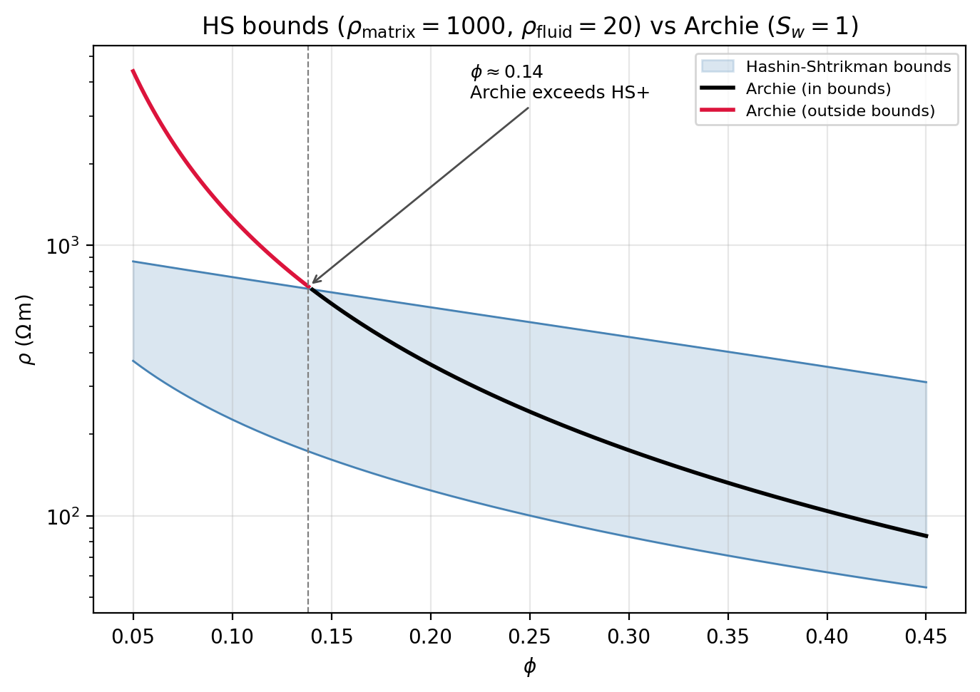
Below roughly 14% porosity, this particular Archie parameterisation
(m=1.8) predicts a resistivity above the Hashin-Shtrikman upper
bound – no microstructure of 1000/20 \(\Omega\mathrm{m}\)
matrix/fluid at that porosity can be that resistive. That does not mean
the rock is impossible; it means this m at this porosity is, and a
lower cementation exponent or a revisited matrix resistivity is needed
before trusting the fit that low.#
in_bounds accepts an optional margin (in log10 ρ) for
cases where being just outside the strict bound by less than typical
measurement uncertainty should not be treated as a hard failure.
8.3.4. Hydraulic conductivity#
Two independent hydraulic-conductivity relationships are relevant to EM sections. Intergranular flow through unconsolidated sediment follows Kozeny-Carman, controlled mainly by grain size and porosity:
>>> from pycsamt.interp.petrophysics import kozeny_carman_K

>>> round(kozeny_carman_K(0.30, d50_m=1e-3), 6)  # 1 mm, coarse sand
0.001502
>>> round(kozeny_carman_K(0.30, d50_m=1e-4), 8)  # 0.1 mm, fine sand
1.502e-05
A tenfold reduction in grain size drops K by two orders of magnitude –
Kozeny-Carman scales with \(d_{50}^2\), so grain size dominates over
porosity for how conductive unconsolidated sediment actually is.
rho_to_hydraulic_conductivity() chains
the whole pipeline – resistivity to porosity via Archie, porosity to K via
Kozeny-Carman – and is only valid where the assumed saturation actually
holds:
>>> from pycsamt.interp.petrophysics import rho_to_hydraulic_conductivity

>>> round(rho_to_hydraulic_conductivity(
...     150.0, archie, rho_w=20.0, phi_prior=0.25, Sw=1.0, d50_m=2.5e-4,
... ), 8)
0.00013065
Fractured basement has no intergranular porosity for Kozeny-Carman to act
on; fractured_zone_K() instead estimates
a fracture volume fraction from the resistivity contrast against intact
matrix rock and applies the parallel-plate cubic law:
>>> from pycsamt.interp.petrophysics import fractured_zone_K

>>> round(fractured_zone_K(1000.0, rho_matrix=5000.0), 6)
0.000654
>>> round(fractured_zone_K(4990.0, rho_matrix=5000.0), 9)
1.635e-06

>>> d50 = np.logspace(np.log10(3e-5), np.log10(6e-3), 100)
>>> K_kc = kozeny_carman_K(0.30, d50_m=d50)
>>> rho_range = np.linspace(10.0, 4990.0, 100)
>>> K_frac = fractured_zone_K(rho_range, rho_matrix=5000.0)

>>> fig, (ax1, ax2) = plt.subplots(1, 2, figsize=(10, 4.5))
>>> _ = ax1.loglog(d50 * 1000, K_kc, color="darkorange")
>>> _ = ax1.set_xlabel("Median grain size $d_{50}$ (mm)")
>>> _ = ax1.set_ylabel("K (m/s)")
>>> _ = ax1.set_title(r"Kozeny-Carman, $\phi=0.30$")
>>> _ = ax1.grid(alpha=0.3, which="both")
>>> _ = ax2.semilogy(rho_range, K_frac, color="teal")
>>> _ = ax2.set_xlabel(r"$\rho$ ($\Omega\,\mathrm{m}$)")
>>> _ = ax2.set_ylabel("K (m/s)")
>>> _ = ax2.set_title(r"Fractured zone, $\rho_\mathrm{matrix}=5000\ \Omega\mathrm{m}$")
>>> _ = ax2.grid(alpha=0.3, which="both")
>>> _ = ax2.invert_xaxis()
>>> fig.tight_layout()
>>> fig.savefig("review/hydraulic_K.png", dpi=200, bbox_inches="tight")
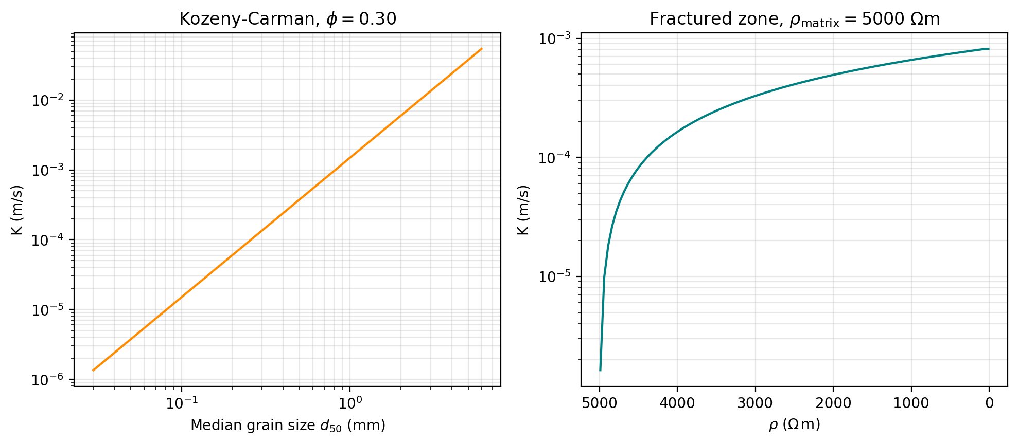
Left: Kozeny-Carman K spans roughly six orders of magnitude across the grain-size range from silty sand to gravel, a straight line on log-log axes confirming the \(d_{50}^2\) scaling. Right: fractured-zone K rises steeply as resistivity drops away from the intact-matrix value (plotted with the x-axis reversed so “more fractured” reads left to right) – the pipeline is a rough first-pass estimate for AMT basement surveys, not a substitute for real fracture characterisation.#
transmissivity()
(Transmissivity) and storativity()
integrate K and porosity over a layer’s saturated thickness –
Hydrogeophysical interpretation already introduces both as
EMHydroModel outputs; called
directly they take plain arrays with no model object involved:
>>> from pycsamt.interp.petrophysics import transmissivity, storativity

>>> round(transmissivity(K=1.5e-4, thickness=25.0), 5)
0.00375
>>> s_confined, s_unconfined = storativity(phi=0.28, thickness=25.0)
>>> s_confined, s_unconfined
(0.0025, 0.28)
storativity always returns both values – confined storativity
\(S=S_s b\) (dimensionless, using specific_storage default
\(10^{-4}\ \mathrm{m^{-1}}\)) and unconfined storativity, approximated
directly as porosity (specific yield). Which one applies depends on
whether the aquifer is actually confined, a judgment the function itself
cannot make from phi/thickness alone.
8.3.5. Pore-water chemistry#
Four short conversions relate pore-water resistivity, electrical conductivity, and total dissolved solids, each with a temperature correction back to a 25 °C reference:
>>> from pycsamt.interp.petrophysics import (
...     rho_w_to_tds, tds_to_rho_w, ec_mscm_to_rho, rho_to_ec_mscm,
... )

>>> round(rho_w_to_tds(20.0), 1)  # fresh groundwater, 25 C
320.0
>>> round(tds_to_rho_w(320.0), 1)
20.0
>>> round(rho_w_to_tds(20.0, temp_c=10.0), 1)
224.0
320 mg/L TDS is comfortably potable (drinking-water guidance is typically
around 500 mg/L); the same 20 \(\Omega\mathrm{m}\) measurement taken at
10 °C instead of 25 °C implies a lower apparent TDS (224 mg/L) purely
from the temperature correction – water is a better conductor when warm,
so an uncorrected cold measurement looks less mineralised than it is.
ec_mscm_to_rho/rho_to_ec_mscm are the same relationship expressed
directly in electrical conductivity (mS/cm) rather than TDS:
>>> round(rho_to_ec_mscm(20.0), 3)
0.5
>>> round(ec_mscm_to_rho(0.5), 1)
20.0
Every pair here round-trips back to its input at 25 °C by construction – useful as a quick self-check when wiring a new pore-water source into a workflow: convert forward and back, and confirm nothing was lost.
8.3.6. EM depth diagnostics#
skin_depth() and
bostick_depth() are the same
calculation under two names – literally the same function call, since
bostick_depth just delegates to skin_depth:
>>> from pycsamt.interp.petrophysics import skin_depth, bostick_depth

>>> round(skin_depth(150.0, freq=1.0), 1)
6164.1
>>> round(skin_depth(150.0, freq=100.0), 1)
616.4
>>> bostick_depth(150.0, freq=1.0) == skin_depth(150.0, freq=1.0)
True
A hundredfold increase in frequency reduces penetration depth by exactly a factor of ten, following the \(\sqrt{1/f}\) scaling in \(\delta=503\sqrt{\rho/f}\). Use this as a sanity check on inversion depth, not a replacement for it: if a model claims resolution at a depth several times beyond the skin depth of its lowest usable frequency, that claim needs scrutiny regardless of what the inversion mesh itself allows.
8.3.7. Profile-based detection#
aquifer_top_from_profile() and
water_table_from_profile() both scan a
1-D resistivity column from the surface down, but they detect different
things and can disagree. aquifer_top_from_profile is a plain threshold
crossing; water_table_from_profile inverts each cell through Archie
first and looks for saturation itself. On the same synthetic column:
>>> z = np.array([5.0, 15.0, 30.0, 55.0, 90.0])
>>> rho_ohm_m = np.array([420.0, 180.0, 95.0, 60.0, 40.0])
>>> rho_log10_col = np.log10(rho_ohm_m)

>>> from pycsamt.interp.petrophysics import (
...     aquifer_top_from_profile, water_table_from_profile,
... )

>>> top = aquifer_top_from_profile(
...     rho_log10_col, z, rho_threshold_ohm_m=100.0, direction="low",
... )
>>> top
30.0
>>> wt = water_table_from_profile(
...     rho_log10_col, z, archie, rho_w=20.0, Sw_threshold=0.85,
... )
>>> wt
15.0
The threshold detector only fires once resistivity actually drops to 100
\(\Omega\mathrm{m}\) or below, at 30 m. The Archie-based detector fires
earlier, at 15 m, because 180 \(\Omega\mathrm{m}\) already implies
\(S_w\ge 0.85\) given phi_prior=0.25 and rho_w=20 – a column
can be “saturated enough” by the Archie criterion well before it crosses a
flat resistivity cutoff. Neither answer is more correct in the abstract;
they encode different definitions of “top of water,” and which one matches
a real drilled water strike is an empirical question for withheld borehole
data, not a property of the algorithm.
>>> fig, ax = plt.subplots(figsize=(5.5, 6))
>>> _ = ax.plot(rho_ohm_m, z, marker="o", color="0.25")
>>> _ = ax.axvline(100.0, color="darkorange", linestyle="--", linewidth=1,
...                 label="aquifer_top threshold (100 $\\Omega$m)")
>>> _ = ax.axhline(top, color="darkorange", linewidth=1.5,
...                 label=f"aquifer_top = {top:.0f} m")
>>> _ = ax.axhline(wt, color="steelblue", linewidth=1.5,
...                 label=f"water_table = {wt:.0f} m")
>>> _ = ax.set_xscale("log")
>>> _ = ax.set_ylim(z.max() + 10, 0)
>>> _ = ax.set_xlabel(r"$\rho$ ($\Omega\,\mathrm{m}$)")
>>> _ = ax.set_ylabel("Depth (m)")
>>> _ = ax.set_title("Threshold crossing vs Archie-$S_w$ detection")
>>> _ = ax.legend(fontsize=8, loc="lower left")
>>> _ = ax.grid(alpha=0.3)
>>> fig.tight_layout()
>>> fig.savefig("review/profile_detection.png", dpi=200, bbox_inches="tight")
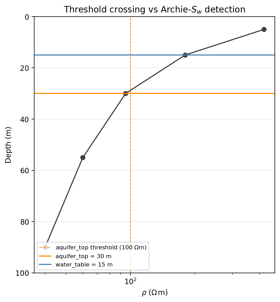
The two detectors read the same profile and disagree by 15 m. Treat either as a hypothesis for field verification, never as a measured water-table depth.#
Warning
Both functions return plain None – not nan – when no
qualifying transition is found in the profile:
>>> flat_rho = np.log10(np.array([2000.0, 1800.0, 1500.0, 1200.0, 1000.0]))
>>> aquifer_top_from_profile(flat_rho, z, rho_threshold_ohm_m=100.0) is None
True
>>> water_table_from_profile(flat_rho, z, archie, rho_w=20.0) is None
True
Code that stores results in a numpy array of dtype float will
silently upcast None to nan on assignment, which is usually
what you want for downstream nanmean/nanmax handling – but a
direct is None check (as above) is required if the distinction
between “searched and found nothing” and “not yet computed” matters.
8.3.8. Next steps#
Continue with:
Hydrogeophysical interpretation for how
ArchieModel,WaxmanSmitsModel, and the hydraulic-conductivity chain combine into a fullEMHydroModelrun over a 2-D section;Uncertainty and validation for how these same models propagate through
MonteCarloHydrowhenm,n,rho_w, ord50_mare themselves uncertain;Lithology classification for the classification engine these petrophysical transforms complement rather than replace;
Interpretation workflow for where petrophysical results fit in the broader review and export pipeline.