
8.5. Monitoring and fusion#
Every other page in this guide treats a resistivity model as one
reviewed snapshot. Two capabilities extend that to more than one model at
once: pycsamt.interp.timelapse compares repeat surveys of the
same profile over time to detect hydrogeological change, and
pycsamt.interp.fusion merges different EM methods – each
sensitive to a different depth window – onto one depth grid. Both are
mentioned only in passing in Hydrogeophysical interpretation; this page works
through them directly.
8.5.1. Grid compatibility#
Comparing two surveys cell-by-cell only makes sense if they share the same
grid. assert_compatible_grids() checks shape,
x_centers, and z_centers before any difference is computed, and
raises rather than silently comparing cells that do not correspond to the
same location:
>>> import numpy as np
>>> from pycsamt.interp import ResistivityModel
>>> from pycsamt.interp.timelapse import assert_compatible_grids

>>> x_m = np.array([0.0, 250.0, 500.0, 750.0, 1000.0])
>>> z_m = np.array([5.0, 15.0, 30.0, 55.0, 90.0])
>>> rho_flat = np.full((5, 5), 100.0)

>>> m1 = ResistivityModel.from_array(np.log10(rho_flat), x_m, z_m, method="TDEM")
>>> z_m_shifted = np.array([5.0, 15.0, 30.0, 55.0, 95.0])
>>> m2 = ResistivityModel.from_array(np.log10(rho_flat), x_m, z_m_shifted, method="TDEM")

>>> try:
...     assert_compatible_grids([m1, m2])
... except ValueError as exc:
...     print(exc)
Survey 1 z_centers differ from survey 0 by more than rtol=0.0001.
A five-metre difference in the deepest cell is enough to raise, because it
means every depth cell below the shallowest few no longer lines up between
the two surveys. TimeLapseEM calls this check
automatically in its constructor – there is no way to build a time-lapse
sequence from incompatible surveys by accident.
8.5.2. Time-lapse differencing#
Building a realistic monitoring sequence: a “dry” baseline, a “wet” survey with patchy recharge strongest near the middle station, and a “recharge” survey where that same patch has wetted further:
>>> rho_dry = np.array([
...     [420.0, 380.0, 350.0, 380.0, 420.0],
...     [380.0, 340.0, 300.0, 340.0, 380.0],
...     [300.0, 260.0, 230.0, 260.0, 300.0],
...     [500.0, 450.0, 420.0, 450.0, 500.0],
...     [1800.0, 1500.0, 1200.0, 1500.0, 1800.0],
... ])
>>> lateral = np.array([0.85, 0.65, 0.45, 0.65, 0.85])
>>> depth_weight = np.array([0.55, 0.45, 0.75, 1.0, 1.0])
>>> mult_wet = 1 - (1 - lateral[None, :]) * depth_weight[:, None] * 0.8
>>> mult_recharge = np.clip(
...     1 - (1 - lateral[None, :]) * depth_weight[:, None] * 1.15, 0.15, None,
... )
>>> rho_wet = rho_dry * mult_wet
>>> rho_recharge = rho_dry * mult_recharge

>>> names = ["S00", "S01", "S02", "S03", "S04"]
>>> model_dry = ResistivityModel.from_array(
...     np.log10(rho_dry), x_m, z_m, station_x=x_m,
...     station_names=names, method="TDEM", rms=1.4,
... )
>>> model_wet = ResistivityModel.from_array(
...     np.log10(rho_wet), x_m, z_m, station_x=x_m,
...     station_names=names, method="TDEM", rms=1.3,
... )
>>> model_recharge = ResistivityModel.from_array(
...     np.log10(rho_recharge), x_m, z_m, station_x=x_m,
...     station_names=names, method="TDEM", rms=1.5,
... )

>>> from pycsamt.interp.timelapse import TimeLapseEM

>>> tl = TimeLapseEM(
...     [model_dry, model_wet, model_recharge],
...     labels=["dry2023", "wet2024", "recharge2024"],
... )
>>> tl
TimeLapseEM(n_surveys=3, n_z=5, n_x=5, labels=['dry2023', 'wet2024', 'recharge2024'])
resistivity_change returns one array per non-baseline survey, always
relative to baseline_idx (default the first survey), never between
consecutive pairs:
>>> delta_rho = tl.resistivity_change()
>>> len(delta_rho)
2
>>> np.round(delta_rho[0], 3)
array([[-0.03 , -0.073, -0.12 , -0.073, -0.03 ],
       [-0.024, -0.058, -0.096, -0.058, -0.024],
       [-0.041, -0.102, -0.174, -0.102, -0.041],
       [-0.056, -0.143, -0.252, -0.143, -0.056],
       [-0.056, -0.143, -0.252, -0.143, -0.056]])
Negative \(\Delta\log_{10}\rho\) means resistivity dropped – wetting,
by the sign convention documented on
resistivity_change(). The
strongest response sits in the middle column (station S02), exactly where
lateral was built to weight it most, and grows from delta_rho[0]
(wet) to delta_rho[1] (recharge) at every depth – a real, monotonic
signal, not noise.
PlotTimeLapseSection renders one such
comparison as a section:
>>> import matplotlib.pyplot as plt
>>> from pycsamt.interp.plot import PlotTimeLapseSection

>>> fig = PlotTimeLapseSection(tl, quantity="rho", survey_idx=1).plot()
>>> fig.savefig("review/timelapse_section.png", dpi=200, bbox_inches="tight")
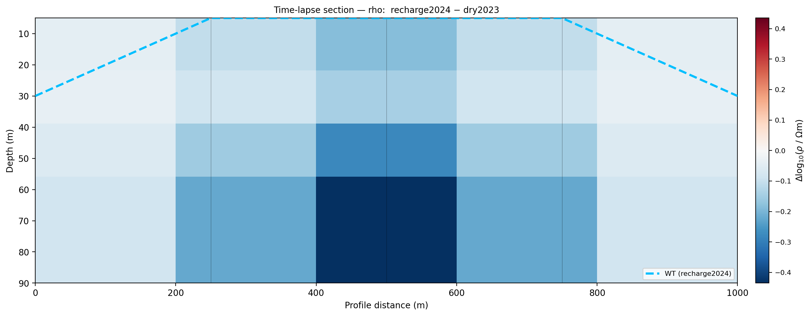
survey_idx=1 selects the second non-baseline survey – recharge,
not wet – since survey_idx indexes into the surveys with the
baseline already excluded. The patchy conductive zone (blue) centred on
station S02 matches the lateral weighting built into the fixture,
and the dashed water-table overlay (from
water_table_from_profile() on the
comparison survey) rises toward the same location.#
8.5.3. From resistivity to hydrology#
A resistivity change alone does not say how much water moved.
saturation_change and water_content_change route each survey
through ArchieModel first, exactly
like Hydrogeophysical interpretation’s single-survey workflow, but applied to every
survey in the sequence:
>>> from pycsamt.interp.petrophysics import ArchieModel

>>> archie = ArchieModel(m=1.8, n=2.0, a=1.0)
>>> delta_sw = tl.saturation_change(archie, phi=0.25, rho_w=20.0)
>>> np.round(delta_sw[0], 3)
array([[0.026, 0.07 , 0.124, 0.07 , 0.026],
       [0.022, 0.059, 0.101, 0.059, 0.022],
       [0.043, 0.034, 0.   , 0.034, 0.043],
       [0.046, 0.131, 0.24 , 0.131, 0.046],
       [0.024, 0.072, 0.151, 0.072, 0.024]])

>>> delta_theta = tl.water_content_change(archie, phi=0.25, rho_w=20.0)
>>> round(float(delta_theta[0][0, 2]), 3)
0.031
At the shallowest cell under station S02 (row 0, column 2) saturation rose
by 0.124 and, multiplied by the assumed porosity of 0.25, the volumetric
water content rose by 0.031 – roughly 3% of the rock volume, by the
fixture’s own assumptions. water_table_displacement and
water_table_map take this further, converting each column into a
single depth using
water_table_from_profile():
>>> wt_map = tl.water_table_map(archie, rho_w=20.0, Sw_threshold=0.85)
>>> wt_map
array([[30., 30., 15., 30., 30.],
       [30.,  5.,  5.,  5., 30.],
       [30.,  5.,  5.,  5., 30.]])

>>> wt_disp = tl.water_table_displacement(archie, rho_w=20.0, Sw_threshold=0.85)
>>> wt_disp
array([[  0., -25., -10., -25.,   0.],
       [  0., -25., -10., -25.,   0.]])
Negative displacement means the water table rose (shallower) – consistent
with recharge, and with the sign convention documented on
water_table_displacement()
(positive = dropped, negative = rose).
>>> fig, ax = plt.subplots(figsize=(6.5, 4.5))
>>> for i, label in enumerate(tl.labels):
...     _ = ax.plot(x_m, wt_map[i], marker="o", label=label)
>>> _ = ax.invert_yaxis()
>>> _ = ax.set_xlabel("Profile distance (m)")
>>> _ = ax.set_ylabel("Water-table depth (m)")
>>> _ = ax.set_title("water_table_map() across the monitoring sequence")
>>> _ = ax.legend(fontsize=8)
>>> _ = ax.grid(alpha=0.3)
>>> fig.tight_layout()
>>> fig.savefig("review/water_table_hydrograph.png", dpi=200, bbox_inches="tight")
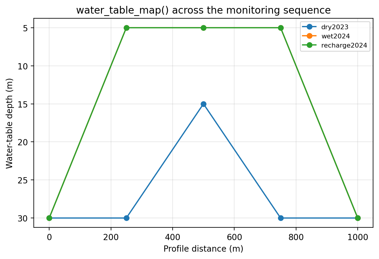
The wet and recharge curves overlap exactly at every station where the water table was detected at all – not what the underlying resistivity change looks like, as the warning below explains.#
Warning
That overlap is not a coincidence of this fixture – it is a real
detection-floor effect. Once a column’s shallowest model cell already
satisfies Sw_threshold, water_table_from_profile cannot report
anything shallower than that cell, no matter how much further the
saturation behind it continues to rise. Compare wt_map (identical
for wet and recharge at every wetted station) against delta_rho and
delta_sw above (both keep growing from wet to recharge at every
depth): the continuous fields keep tracking additional wetting after
the threshold-based water-table detector has saturated at the mesh’s
shallowest cell. Prefer resistivity_change/saturation_change
over water_table_map when a monitoring signal might continue to
evolve near the surface.
Warning
saturation_change, water_content_change, and
water_table_displacement all accept a
WaxmanSmitsModel in place of
petro, but internally convert it to a plain
ArchieModel using only its m,
n, and a – sigma_s (clay conductivity) is silently
dropped:
>>> from pycsamt.interp.petrophysics import WaxmanSmitsModel

>>> ws = WaxmanSmitsModel(m=1.8, n=2.0, a=1.0, sigma_s=0.02)
>>> delta_sw_ws = tl.saturation_change(ws, phi=0.25, rho_w=20.0)
>>> delta_sw_archie = tl.saturation_change(
...     ArchieModel(m=1.8, n=2.0, a=1.0), phi=0.25, rho_w=20.0,
... )
>>> bool(np.allclose(delta_sw_ws[0], delta_sw_archie[0]))
True
Passing a calibrated Waxman-Smits model here buys nothing over passing the equivalent Archie model directly – the same approximation already documented for Waxman-Smits model water-table detection in Hydrogeophysical interpretation applies to every time-lapse method in this section.
8.5.4. Monitoring a full sequence#
resistivity_stats summarises change across every non-baseline survey
at once – useful once a sequence has more than two surveys and a single
before/after difference stops telling the whole story:
>>> stats = tl.resistivity_stats()
>>> sorted(stats)
['max_decrease', 'max_increase', 'mean_delta', 'std_delta']
>>> round(float(stats["mean_delta"][2, 2]), 3)
-0.227
>>> round(float(stats["std_delta"][2, 2]), 3)
0.053
At row 2, station S02, the mean change across both comparison surveys is
\(-0.227\) in \(\log_{10}\rho\), with a standard deviation of only
0.053 – the two surveys agree on both the direction and the rough
magnitude of the change, which is what makes this cell a credible
monitoring signal rather than survey-to-survey noise.
PlotMultiTimeLapseGrid lays out the whole
sequence side by side instead of summarising it:
>>> from pycsamt.interp.plot import PlotMultiTimeLapseGrid

>>> fig = PlotMultiTimeLapseGrid(tl, quantity="delta_rho").plot()
>>> fig.savefig("review/multi_grid.png", dpi=200, bbox_inches="tight")
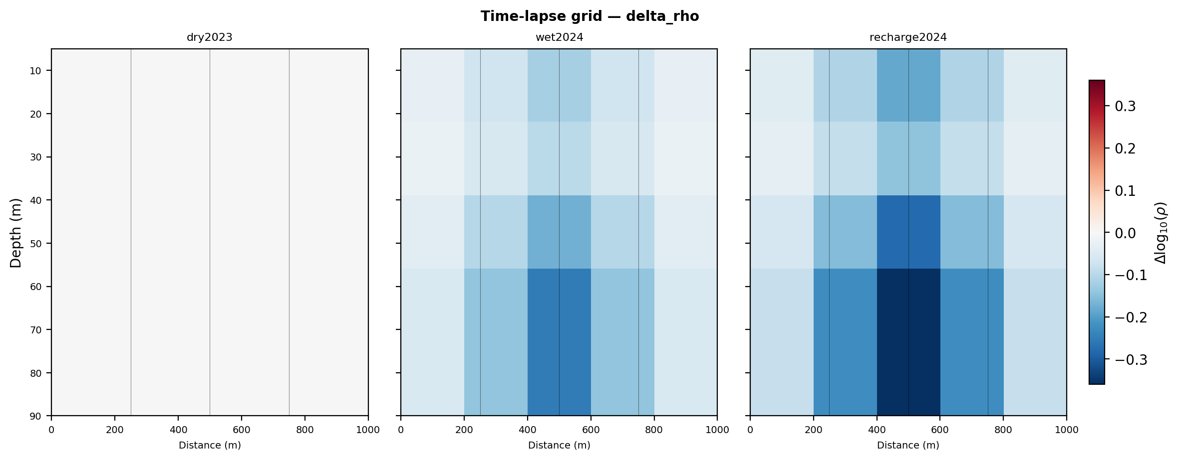
The baseline panel (dry2023) is exactly zero by construction –
plotting a survey against itself as baseline_idx. The anomaly
visibly deepens and strengthens from wet to recharge, giving the same
progression as the mean/std summary above but as a direct visual
comparison rather than two numbers.#
8.5.5. Multi-method fusion#
Different EM methods resolve different depth windows: a TDEM survey might
be trusted from 10-300 m and an AMT survey from 100-1700 m, overlapping
between 100 and 300 m.
MultiMethodEMModel interpolates both onto
one depth grid and blends them in that overlap:
>>> z_tdem = np.array([10.0, 30.0, 60.0, 100.0, 150.0, 220.0, 300.0])
>>> rho_tdem = np.tile(
...     np.array([80.0, 60.0, 45.0, 70.0, 150.0, 400.0, 900.0])[:, None], (1, 5),
... )
>>> tdem = ResistivityModel.from_array(
...     np.log10(rho_tdem), x_m, z_tdem, station_x=x_m, method="TDEM", rms=1.6,
... )
>>> z_amt = np.array([100.0, 200.0, 350.0, 550.0, 800.0, 1200.0, 1700.0])
>>> rho_amt = np.tile(
...     np.array([180.0, 350.0, 700.0, 1200.0, 2500.0, 4000.0, 6000.0])[:, None], (1, 5),
... )
>>> amt = ResistivityModel.from_array(
...     np.log10(rho_amt), x_m, z_amt, station_x=x_m, method="AMT", rms=2.1,
... )

>>> from pycsamt.interp.fusion import MultiMethodEMModel

>>> fm = MultiMethodEMModel(tdem, amt, blend="sigmoid", sigmoid_k=0.03)
>>> fused = fm.merge()
>>> fused.method
'TDEM+AMT'
>>> fused.z_centers
array([  10.,   30.,   60.,  100.,  150.,  200.,  220.,  300.,  350.,
        550.,  800., 1200., 1700.])
The output depth grid is the union of both models’ depth cells, not a
resampling onto a fixed spacing – merge() never invents a depth cell
that neither source model had. diagnostics_ records what happened:
>>> d = fm.diagnostics_
>>> d.has_overlap, d.z_overlap_start, d.z_overlap_end
(True, 100.0, 300.0)
>>> d.n_z_fused
13
>>> np.round(d.blend_weights, 2)
array([1.  , 1.  , 1.  , 1.  , 0.82, 0.5 , 0.35, 0.  , 0.  , 0.  , 0.  ,
       0.  , 0.  ])
A weight of 1 means pure primary (TDEM); 0 means pure secondary (AMT). Outside 100-300 m the fused model is just one source model reinterpolated onto the union grid, unmodified.
8.5.6. Blend strategies#
The three blend modes only differ inside the overlap zone, and only
become visually distinguishable when probed on a grid finer than the
handful of depth cells the two source models actually contribute –
mapping each mode across a dense depth axis from 50 to 350 m makes the
shape of each strategy visible:
>>> z_probe = np.linspace(50.0, 350.0, 300)
>>> fig, ax = plt.subplots(figsize=(6.5, 4.5))
>>> for blend in ("linear", "sigmoid", "rms_weighted"):
...     fm_i = MultiMethodEMModel(
...         tdem, amt, blend=blend, z_grid=z_probe, sigmoid_k=0.03,
...     )
...     _ = fm_i.merge()
...     _ = ax.plot(z_probe, fm_i.diagnostics_.blend_weights, label=blend)
>>> _ = ax.axvspan(100.0, 300.0, color="0.85", alpha=0.5, label="overlap zone")
>>> _ = ax.set_xlabel("Depth (m)")
>>> _ = ax.set_ylabel("Primary (TDEM) weight")
>>> _ = ax.set_title("Blend weight vs depth, probed on a dense grid")
>>> _ = ax.legend(fontsize=8)
>>> _ = ax.grid(alpha=0.3)
>>> fig.tight_layout()
>>> fig.savefig("review/blend_weights.png", dpi=200, bbox_inches="tight")
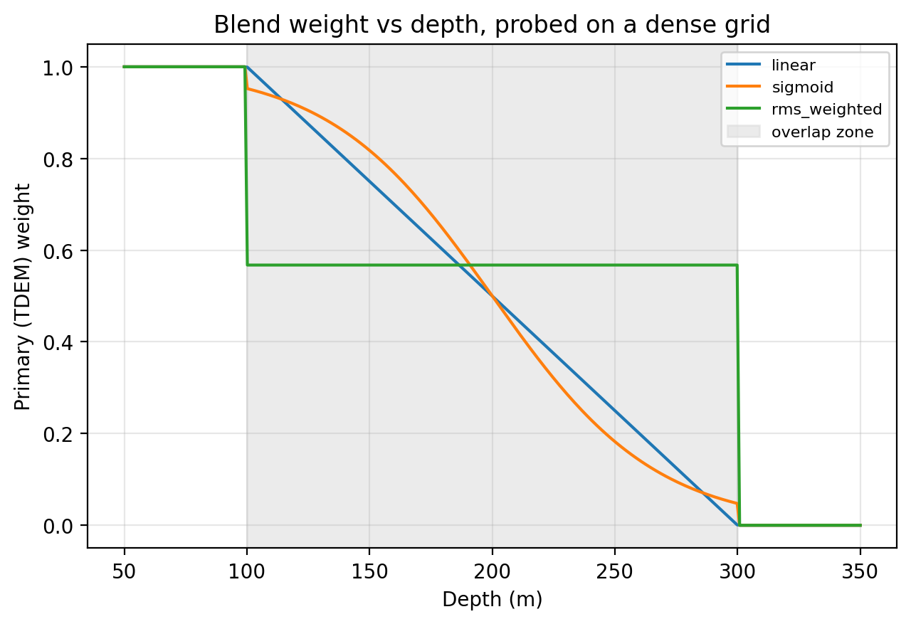
linear and sigmoid both ramp smoothly from 1 to 0 across the
overlap – sigmoid simply flattens the ends and steepens the
middle. rms_weighted is not a ramp at all: it holds one constant
weight (here rms_amt / (rms_tdem + rms_amt) ≈ 0.57) across the
entire overlap and steps abruptly to 1 and 0 at the overlap’s edges.
Choosing rms_weighted expecting a smooth transition like the other
two modes will produce visible discontinuities in a fused section at
both overlap boundaries.#
On the natural (non-probed) grid, the fused profile at one station shows why the overlap matters at all – the two source curves visibly disagree about resistivity in their shared depth range, and the fused curve is the compromise the blend weights produce, not either source curve alone:
>>> ix = 2  # station S02
>>> fig, ax = plt.subplots(figsize=(5.5, 6))
>>> _ = ax.plot(10.0 ** tdem.rho_2d[:, ix], tdem.z_centers, "o-",
...              color="darkorange", label="TDEM (primary)")
>>> _ = ax.plot(10.0 ** amt.rho_2d[:, ix], amt.z_centers, "o-",
...              color="steelblue", label="AMT (secondary)")
>>> _ = ax.plot(10.0 ** fused.rho_2d[:, ix], fused.z_centers, "-",
...              color="black", linewidth=2, label="fused")
>>> _ = ax.axhspan(100.0, 300.0, color="0.85", alpha=0.4, zorder=0)
>>> _ = ax.set_xscale("log")
>>> _ = ax.set_ylim(1800, 5)
>>> _ = ax.set_xlabel(r"$\rho$ ($\Omega\,\mathrm{m}$)")
>>> _ = ax.set_ylabel("Depth (m)")
>>> _ = ax.set_title("Station S02 -- primary, secondary, and fused")
>>> _ = ax.legend(fontsize=8)
>>> _ = ax.grid(alpha=0.3)
>>> fig.tight_layout()
>>> fig.savefig("review/fused_profile.png", dpi=200, bbox_inches="tight")
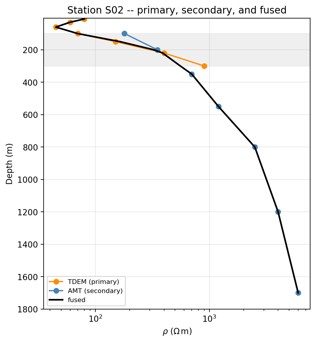
TDEM and AMT already roughly agree near 200 m, which is why the fused curve barely bends through the shaded overlap; a wider disagreement there would show up as a sharper corner in the fused curve rather than an actual physical layer boundary. Reading a fusion-zone kink as geology instead of as a blend artefact is the most common misreading of a fused section.#
8.5.7. Fusion edge cases#
Two behaviours are worth checking deliberately rather than discovering
under deadline. When the two depth ranges genuinely do not overlap,
merge() falls back to a hard boundary rather than blending anything:
>>> z_tdem_shallow = np.array([10.0, 30.0, 60.0, 90.0])
>>> rho_tdem_shallow = np.tile(
...     np.array([80.0, 60.0, 45.0, 70.0])[:, None], (1, 5),
... )
>>> tdem_shallow = ResistivityModel.from_array(
...     np.log10(rho_tdem_shallow), x_m, z_tdem_shallow,
...     station_x=x_m, method="TDEM", rms=1.6,
... )
>>> z_amt_deep = np.array([150.0, 300.0, 600.0])
>>> rho_amt_deep = np.tile(
...     np.array([300.0, 1000.0, 3000.0])[:, None], (1, 5),
... )
>>> amt_deep = ResistivityModel.from_array(
...     np.log10(rho_amt_deep), x_m, z_amt_deep,
...     station_x=x_m, method="AMT", rms=2.0,
... )

>>> fm_gap = MultiMethodEMModel(tdem_shallow, amt_deep)
>>> _ = fm_gap.merge()
>>> fm_gap.diagnostics_.has_overlap
False
>>> fm_gap.diagnostics_.blend_weights
array([1., 1., 1., 1., 1., 0., 0.])
With no overlap, every depth up to and including the secondary model’s
shallowest cell (150 m here) takes the primary value, and everything
beyond it takes the secondary value – there is no transition zone to
blend across, so blend has no effect at all in this configuration.
The second behaviour is a documented fallback, and it holds up under a
direct check: blend="rms_weighted" needs a finite rms on both
models, and silently reduces to "linear" when either is nan:
>>> tdem_nanrms = tdem.clone(rms=float("nan"))
>>> fm_nan = MultiMethodEMModel(tdem_nanrms, amt, blend="rms_weighted")
>>> _ = fm_nan.merge()
>>> fm_linear = MultiMethodEMModel(tdem, amt, blend="linear")
>>> _ = fm_linear.merge()
>>> bool(np.array_equal(
...     fm_nan.diagnostics_.blend_weights, fm_linear.diagnostics_.blend_weights,
... ))
True
Both models carry an rms precisely because ResistivityModel.
from_occam2d and similar
adapters populate it from real inversion output; a model built with
from_array() and no explicit
rms defaults to nan, which silently steers rms_weighted back
to linear rather than raising – worth checking for if a fused section
looks unexpectedly like a plain linear ramp.
8.5.8. Next steps#
Continue with:
Hydrogeophysical interpretation for the single-survey petrophysical workflow that every method on this page builds on;
Petrophysical toolkit for
ArchieModel/WaxmanSmitsModelmechanics in isolation from any model object;Uncertainty and validation for propagating parameter uncertainty through a single survey – not yet combined with time-lapse or fusion in this guide;
Interpretation workflow for where a fused or time-lapse product fits in the broader review and export pipeline.