18.8. Process A TEMAVG Survey: TEM To Corrected EDI

This tutorial walks a real TEM/TDEM survey from raw field files to a reviewed, corrected EDI collection with a real geographic anchor, on to an inspectable 2-D triangular mesh, and finally to a real, gated Maxwell-physics AI inversion trained on that mesh: read the bundled data/TEMAVG/JIANGSU TEMAVG file folder, quality-control the raw time-domain decay, resolve a geographic coordinate for the local site grid with pycsamt.gis, transform to pseudo-frequency impedance with pycsamt.tdem, apply the same pycsamt.emtools corrections used for frequency-domain surveys, build/draw a real graded, topography- draped mesh with pycsamt.forward.maxwell and pycsamt.api.mesh, and train/gate Inv2DAgent(physics="mt2d_tri") on it, the same in-process TriFEM2DAdapter path Map Groundwater Geology From CSAMT uses. The classical, external-binary route – Prepare A MARE2DEM Inversion’s PSLG triangulation – stays out of scope here.

TDEM Basics derives every formula used below (transient diffusion, the late-time apparent-resistivity approximation, pseudo-frequency conventions, and the noise/error-floor model); this page focuses on the workflow decisions a real survey forces and does not re-derive that physics.

JIANGSU is a station grid, not one line: the coordinate table spans 102 planned 40 m-spaced profiles, but only 55 were actually surveyed and processed into .AVG/.LOG/.Z file triplets. Every example below works one representative profile, TEM100 (51 stations, 20 m spacing, a 1000 m line), the same way Process Zonge AVG Lines K1 and K2 works one line at a time from a larger CSAMT/AMT survey.

18.8.1. Read the survey folder

read_temavg_survey() parses every .AVG file in a folder, groups companion .LOG and .Z files by stem, and looks for a coordinate table using common filenames. The CLI reports the same summary without writing any Python:

$ pycsamt tdem info data/TEMAVG/JIANGSU
Survey root : data\TEMAVG\JIANGSU
AVG files   : 55
  TEM100  (1275 records)
  TEM1020  (1275 records)
  TEM1060  (1275 records)
  ...
Z files     : 55
LOG files   : 55
Coordinates : 5159 points  (with elevation)

Reading this survey’s coordinate table, a legacy Coordinate of measuring point.xls, needs the optional xlrd dependency (pip install "pycsamt[docs]" or pip install xlrd); without it the join is silently skipped and this line reports none found instead of raising, so always check it rather than assuming coordinates loaded.

>>> from pycsamt.tdem import read_temavg_survey
>>> survey = read_temavg_survey("data/TEMAVG/JIANGSU")
>>> survey.n_avg_files, survey.n_z_files, survey.n_log_files
(55, 55, 55)
>>> survey.coordinates.n_points
5159
>>> coords = survey.coordinates.to_dataframe()
>>> coords.profile.nunique(), len(survey.avg_files)
(102, 55)

18.8.2. Pick one profile and inspect its geometry

The file stem’s numeric suffix is the profile id (TEM100 -> profile 100); within one file, TEMAVG’s station column is the along-profile chainage. TEM100 is a genuine central-loop sounding: the Array metadata, the equal TXdx/TXdy, and the mde sidecar’s Line.Azimuth = 90 all agree on an east-west, 360 m square transmitter loop with the receiver at its centre.

>>> avg = survey.get("TEM100")
>>> avg.metadata
{'title': 'TEMAVG 7.77: "TEM100.FLD", Dated 21-07-04, Processed 24 Oct 24',
 'Array': 'In Loop (Central Loop)', 'TXramp': 450, 'TXdx': 360,
 'TXdy': 360, 'TXarea': 129600, 'RXarea': 10000}
>>> len(avg.stations), avg.n_records
(51, 1275)
>>> avg.stations[0], avg.stations[-1]
(100.0, 1100.0)
>>> soundings = survey.to_soundings(stems=["TEM100"])
>>> soundings[0].moment  # M = I * n_tx * A_tx
1296000.0

</>View the executed survey-map and topography figure codeClick to inspect and copy the complete code

def make_survey_overview(survey, avg, soundings) -> Path:
    """Plot the full station grid and the TEM100 elevation profile."""
    coords = survey.coordinates.to_dataframe()
    line = coords[coords.profile == float(_profile_number(PROFILE_STEM))]
    line = line.sort_values("point")

    fig, axes = plt.subplots(1, 2, figsize=(11.5, 4.6), constrained_layout=True)

    ax = axes[0]
    ax.scatter(
        coords.gauss_y, coords.gauss_x, s=2, c="#b0b0b0", label="planned grid pegs"
    )
    ax.scatter(
        line.gauss_y, line.gauss_x, s=14, c="#d62728", label=f"{PROFILE_STEM} stations"
    )
    ax.set(
        title=f"JIANGSU grid: {len(survey.avg_files)} surveyed profiles of "
        f"{coords.profile.nunique()} planned",
        # Chinese Gauss-Krüger convention: X = northing, Y = zone-prefixed
        # easting -- the opposite of the usual (easting, northing) reading.
        xlabel="Gauss-Krüger Y (zone-prefixed easting, m)",
        ylabel="Gauss-Krüger X (northing, m)",
    )
    ax.ticklabel_format(useOffset=False, style="plain")
    ax.legend(fontsize=8)
    ax.grid(alpha=0.25)

    ax = axes[1]
    ax.plot(line.point, line.elevation, "o-", ms=3.5, color="#1f77b4")
    ax.set(
        title=f"{PROFILE_STEM}: measured topography ({len(line)} stations)",
        xlabel="Station chainage (m)",
        ylabel="Elevation (m)",
    )
    ax.grid(alpha=0.25)

    target = OUT / "jiangsu_survey_overview.png"
    fig.savefig(target, dpi=180)
    plt.close(fig)
    return target

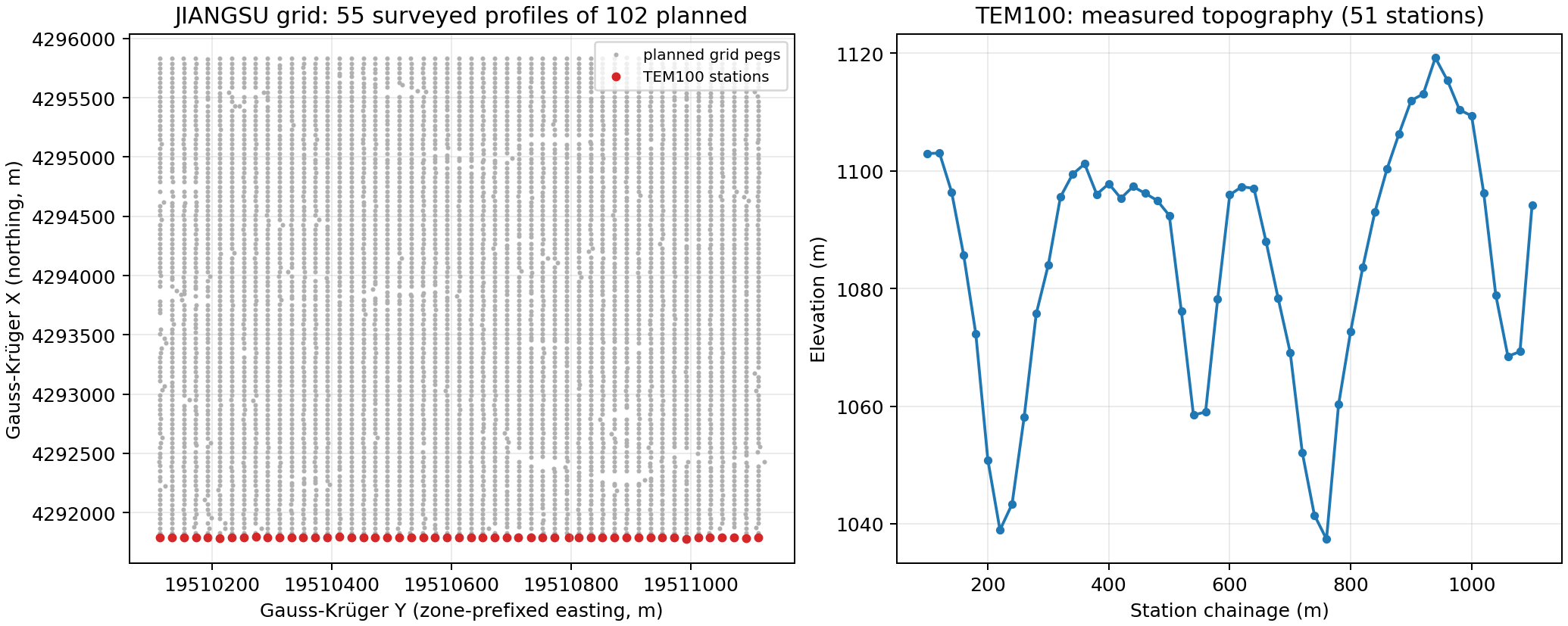
Left: 55 of 102 planned profiles were actually surveyed; TEM100 (red) is the southernmost, running east-west along nearly constant Gauss-Krüger X (northing). Right: TEM100’s 51 stations cross about 82 m of relief (1037-1119 m) over the 1000 m line – real topography that a later inversion mesh needs to honour, not a flat-earth convenience.

18.8.3. Quality-control the raw time-domain decay before transforming

TDEM Basics warns generically against “interpreting noisy late gates” and “dropping sign information without documenting why.” TEM100 shows exactly the pattern that warning is about. TEMAVG’s magnitude column is signed; a negative value at late time means the stacked transient crossed zero, i.e. the signal has fallen into the noise floor before that gate. The late-time formula only ever sees |dBdt|, so feeding a sign-flipped gate through it does not raise an error – it silently fabricates an apparent resistivity from noise.

>>> import numpy as np
>>> mag = np.array([rec.magnitude for rec in avg.records])
>>> win = np.array([rec.window for rec in avg.records])
>>> pct = np.array([rec.percent_magnitude for rec in avg.records])
>>> int((mag < 0).sum()), len(mag)
(49, 1275)
>>> round(float(pct.max()), 1)  # the %Mag column alone never flags these
18.0
>>> [(w, int(((win == w) & (mag < 0)).sum())) for w in range(20, 26)]
[(20, 1), (21, 2), (22, 4), (23, 10), (24, 9), (25, 18)]

The percent-magnitude column – the closest thing TEMAVG provides to a native error estimate – never exceeds 18% anywhere in this file, so a threshold on it alone would not catch a single one of these 49 rows. Only the sign is diagnostic here, and it grows sharply at the last three windows: by window 25 (the latest gate, 12.2 ms), 18 of 51 stations have gone negative.

</>View the executed decay-curve and per-window QC figure codeClick to inspect and copy the complete code

def make_time_domain_qc(avg, soundings) -> tuple[Path, dict]:
    """Plot signed decay curves and the per-window sign-reversal count."""
    n_windows = max(rec.window for rec in avg.records)
    neg_count = np.zeros(n_windows, dtype=int)
    for rec in avg.records:
        if rec.magnitude < 0.0:
            neg_count[rec.window - 1] += 1
    n_stations = len(avg.stations)

    picks = [soundings[0], soundings[len(soundings) // 2], soundings[-1]]

    fig, axes = plt.subplots(1, 2, figsize=(11.5, 4.6), constrained_layout=True)

    ax = axes[0]
    for snd in picks:
        t_ms = snd.time_gates * 1e3
        pos = snd.data > 0.0
        ax.loglog(t_ms[pos], snd.data[pos], "o-", ms=4, lw=1.2, label=snd.station_name)
        if (~pos).any():
            ax.loglog(
                t_ms[~pos],
                np.abs(snd.data[~pos]),
                "x",
                ms=9,
                mew=2,
                color="black",
                label="_nolegend_",
            )
    ax.set(
        title="Signed decay curves (x = negative magnitude)",
        xlabel="Time (ms)",
        ylabel="|processed magnitude| (V)",
    )
    ax.grid(True, which="both", alpha=0.3)
    ax.legend(fontsize=8)

    ax = axes[1]
    ax.bar(np.arange(1, n_windows + 1), neg_count, color="#d62728")
    ax.set(
        title=f"{PROFILE_STEM}: stations with negative magnitude per window",
        xlabel="Time-window number",
        ylabel=f"Station count (of {n_stations})",
    )
    ax.grid(alpha=0.25, axis="y")

    target = OUT / "tem100_time_domain_qc.png"
    fig.savefig(target, dpi=180)
    plt.close(fig)

    stats = {
        "n_windows": n_windows,
        "neg_count_per_window": neg_count,
        "n_stations": n_stations,
        "n_records": len(avg.records),
        "n_negative_total": int(neg_count.sum()),
    }
    return target, stats

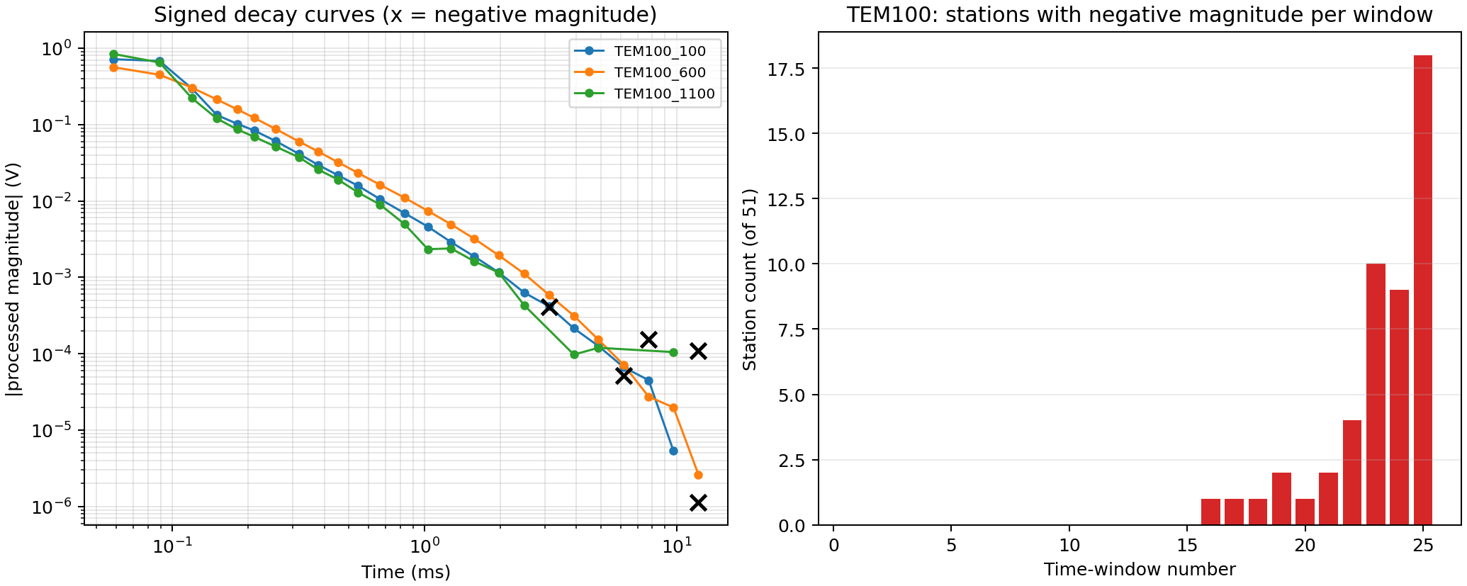
Left: three representative stations follow the expected power-law decay for four decades before the marked (x) gates flip sign near the noise floor. Right: sign reversals are essentially absent before window 16 and climb steeply after window 21 – a station-dependent, not a fixed-window, effect.

The decision applied throughout the rest of this page is to drop each station’s own negative-magnitude gates before transforming, rather than applying a single blanket window cutoff to every station or, worse, silently abs()-ing them into the late-time formula:

</>View the noise-floor gate-drop functionClick to inspect and copy the complete code

def drop_noise_floor_gates(snd: TEMSounding) -> tuple[TEMSounding, int]:
    """Remove gates whose processed magnitude is negative.

    A negative TEMAVG ``magnitude`` at late time means the stacked
    transient has crossed zero -- the signal has fallen into the noise
    floor and the sign is not physically meaningful for the late-time
    apparent-resistivity formula, which only ever sees ``|dBdt|``. Feeding
    those gates in unfiltered does not raise an error; it silently
    fabricates a resistivity value from noise.
    """
    keep = snd.data > 0.0
    n_dropped = int((~keep).sum())
    cleaned = TEMSounding(
        time_gates=snd.time_gates[keep],
        data=snd.data[keep],
        current=snd.current,
        tx_area=snd.tx_area,
        data_type=snd.data_type,
        tx_turns=snd.tx_turns,
        rx_area=snd.rx_area,
        rx_turns=snd.rx_turns,
        offset=snd.offset,
        loop_shape=snd.loop_shape,
        loop_dims=snd.loop_dims,
        station_name=snd.station_name,
        x=snd.x,
        y=snd.y,
        elevation=snd.elevation,
        error=(snd.error[keep] if snd.error is not None else None),
        waveform=snd.waveform,
    )
    return cleaned, n_dropped

>>> from docs.scripts.generate_tutorial_temavg_workflow import drop_noise_floor_gates
>>> cleaned = [drop_noise_floor_gates(s)[0] for s in soundings]
>>> n_dropped = sum(drop_noise_floor_gates(s)[1] for s in soundings)
>>> n_dropped, sum(s.n_gates for s in soundings)
(49, 1275)
>>> min(s.n_gates for s in cleaned), max(s.n_gates for s in cleaned)
(15, 25)

One station loses 10 of its 25 gates this way; most lose zero or one. This trims the deepest nominal sensitivity where the trimming happens (dropping gate 25 removes the lowest pseudo-frequency point specifically), a real trade-off against keeping fabricated late-time values – not a free QC step.

18.8.4. Determine a geographic anchor for the local site grid

The coordinate table carries two coordinate pairs per station: a local x/y (the small numbers used so far, ~100 m scale, matching station chainage) and a projected gauss_x/gauss_y pair in the millions – Chinese Gauss-Krüger convention, with the zone number folded into gauss_y as a zone * 1,000,000 prefix. Neither is geographic lat/lon, and unlike Process Zonge AVG Lines K1 and K2’s K1/K2 lines (whose EPSG:32649 provenance was already known), no CRS is documented for this survey. It has to be inferred, and checked, before it is used.

>>> y = coords.gauss_y.iloc[0]
>>> zone = int(y // 1_000_000)
>>> zone  # embedded in every gauss_y value
19

pyCSAMT registers this zone under several historical and modern Chinese datums; CGCS2000 / Gauss-Kruger zone 19 (EPSG:4497) is the current standard one:

>>> from pycsamt.gis.utils import epsg_project
>>> lon, lat = epsg_project(y, coords.gauss_x.iloc[0], 4497, 4326)
>>> round(lon, 4), round(lat, 4)
(111.1163, 38.7593)

That coordinate is not in Jiangsu – it is roughly 38.8°N, 111.1°E, near the Shanxi/Shaanxi border, about 8 degrees of latitude (nearly 900 km) north of Jiangsu province (30.75-35.2°N). Zone 19 itself only fixes the column of longitude (108-114°E per its EPSG area of use); the northing value fixes latitude independent of which zone-19 CRS is chosen, and every CGCS2000/Xian80/Beijing54 zone-19 candidate lands in the same place. The survey’s elevations (1037-1119 m) are equally inconsistent with Jiangsu’s real topography, a mostly flat coastal plain rarely above a few hundred metres. Both independent checks point the same way: gauss_x/gauss_y reads as a local site grid with an arbitrary large false origin – common practice for Chinese mineral-exploration TEM contractors, and not unusual when a crew has no RTK tie to the national datum on site – rather than true national Gauss-Krüger coordinates. The “JIANGSU” folder name is provenance for the delivery, not evidence for this specific claim.

This is exactly the kind of gap this documentation build does not paper over by default. Here it is used anyway, because a geographic anchor is more useful for the mesh and manifest work below than none, provided it is labelled for what it is: an explicit best-effort guess, not a verified survey location.

</>View the executed coordinate-projection codeClick to inspect and copy the complete code

def attach_geographic_coords(soundings, survey, *, epsg: int = GK_EPSG):
    """Overwrite each sounding's local x/y with projected lon/lat.

    Uses :func:`pycsamt.gis.utils.epsg_project` on the coordinate table's
    ``gauss_x``/``gauss_y`` (already zone-prefixed, so no manual false-
    easting arithmetic is needed). This is a best-effort geographic anchor,
    not a verified one -- see :data:`GK_EPSG`.
    """
    from pycsamt.gis.utils import epsg_project

    for snd in soundings:
        stem, station = snd.station_name.split("_")
        profile = float("".join(ch for ch in stem if ch.isdigit()))
        coord = survey.coordinates.get(profile, float(station))
        if coord is None:
            continue
        lon, lat = epsg_project(coord.gauss_y, coord.gauss_x, epsg, 4326)
        snd.x, snd.y = float(lon), float(lat)
    return soundings

>>> from docs.scripts.generate_tutorial_temavg_workflow import attach_geographic_coords
>>> _ = attach_geographic_coords(soundings, survey)  # mutates in place
>>> soundings[0].x, soundings[0].y  # now lon, lat -- not local metres
(111.11634836490072, 38.75930206136827)

18.8.5. Transform to frequency domain and write EDI

TEMtoEDI wraps LateTimeTransform (used here; FourierTransform needs a captured transmitter waveform, which this AVG file does not carry, exactly the limitation TDEM Basics documents) and writes one synthetic EDI per station. Because only Hz was measured, every EDI carries a single independent transfer function: \(Z_{xx}=Z_{yy}=0\) and \(Z_{yx}=-Z_{xy}\), with phase fixed at the default homogeneous \(45^\circ\) rather than measured – the same single-component limitation Process Zonge AVG Lines K1 and K2 documents for the Ex-Hy-only K1/K2 lines, here even more synthetic since even \(Z_{xy}\) itself is derived from one decay curve rather than an independently recorded electric channel.

</>View the executed clean -> transform -> write -> reload codeClick to inspect and copy the complete code

def convert_profile_to_edi(soundings, out_dir: Path):
    """Drop noise-floor gates, transform to EDI, write, and reload."""
    from pycsamt.emtools import ensure_sites

    cleaned, n_dropped = [], 0
    for snd in soundings:
        c, n = drop_noise_floor_gates(snd)
        cleaned.append(c)
        n_dropped += n

    conv = TEMtoEDI(method="late_time", phase_mode="homogeneous", out_dir=str(out_dir))
    written = conv.save(cleaned)
    sites = ensure_sites(out_dir, recursive=False).ordered(by="station")

    stats = {
        "n_dropped_total": n_dropped,
        "n_gates_in": sum(s.n_gates for s in soundings),
        "n_written": len(written),
        "n_reloaded": len(sites),
        "n_gates_out_min": min(len(s.freq) for s in sites),
        "n_gates_out_max": max(len(s.freq) for s in sites),
    }
    return sites, stats

>>> from docs.scripts.generate_tutorial_temavg_workflow import convert_profile_to_edi, RESULTS
>>> raw_sites, stats = convert_profile_to_edi(soundings, RESULTS / "edi_raw" / "TEM100")
>>> stats
{'n_dropped_total': 49, 'n_gates_in': 1275, 'n_written': 51,
 'n_reloaded': 51, 'n_gates_out_min': 15, 'n_gates_out_max': 25}
>>> raw_sites[0].coords  # (lat, lon, elev), real now, not NaN
(38.759302777777776, 111.11634722222222, 1102.9537)

The CLI equivalent for a full survey folder (or, with --stems, one profile) is:

$ pycsamt tdem convert data/TEMAVG/JIANGSU --stems TEM100 --dry-run
Dry run — 51 sounding(s) would be converted:
  TEM100_100
  TEM100_120
  TEM100_140
  ...
  TEM100_1080
  TEM100_1100

$ pycsamt tdem convert data/TEMAVG/JIANGSU --stems TEM100 \
    --output-dir results/process_temavg_survey/edi_raw/TEM100

The CLI path above skips the coordinate-projection step, so it writes HEAD with the raw local x/y from the coordinate table; those values are outside geographic bounds (y up to 1100), so TEMtoEDI leaves LAT/LONG unset rather than writing an invalid geographic coordinate, and records the local values as an INFO note instead. The Python path above is what actually gets a (best-effort) geographic coordinate into HEAD, because it runs attach_geographic_coords() first.

One further detail of this write/reload round trip is worth stating explicitly: Site.rho/Site.phase reload correctly because TEMtoEDI builds \(|Z_{xy}|\) with pyCSAMT’s own field-unit EDI convention, \(|Z|=\sqrt{5f\rho_a}\) (the same one pycsamt.z.resphase.ResPhase.compute_resistivity_phase() uses to read resistivity back out) – not the SI convention \(|Z|=\sqrt{\rho_a\omega\mu_0}\), which shares the same TDEM Basics late-time derivation but is not what the rest of pyCSAMT’s EDI stack expects when it reads Z back off disk.

18.8.6. Correct the EDI collection

The same single-component limitation from the previous section rules out phase-tensor, skew, and strike diagnostics here for the same reason Process Zonge AVG Lines K1 and K2 gives for K1/K2: \(\operatorname{Re}\mathbf Z\) is singular with only one measured off-diagonal entry. What is applicable is the same two-stage frequency-domain conditioning used there: a Hampel despike in magnitude/phase space, then the Torres-Verdín-Bostick Hanning spatial filter for static shift, this time over the real 20 m station spacing.

</>View the executed Hampel + static-shift correction codeClick to inspect and copy the complete code

def make_edi_processing(raw_sites):
    """Apply Hampel despiking and Hanning static-shift correction."""
    from pycsamt.emtools import correct_static_shift, hampel_filter_freq

    despiked = hampel_filter_freq(
        raw_sites, win=2, nsig=3.0, on="z", domain="magphase", inplace=False
    )
    n_cells_total = 0
    n_cells_changed = 0
    for a, b in zip(raw_sites, despiked):
        za, zb = a.z[..., 0, 1], b.z[..., 0, 1]
        n_cells_total += za.size
        n_cells_changed += int(np.sum(~np.isclose(za, zb, equal_nan=True)))

    corrected = correct_static_shift(
        despiked, window_m=200.0, spacing_m=20.0, comp="xy", inplace=False
    )

    station = np.array([float(s.name.split("_")[1]) for s in raw_sites])
    freq_common = np.unique(np.concatenate([s.freq for s in raw_sites]))
    freq_common.sort()

    def _grid(sites):
        grid = np.full((len(sites), freq_common.size), np.nan)
        for i, s in enumerate(sites):
            rho = s.rho[..., 0, 1]
            idx = np.searchsorted(freq_common, s.freq)
            grid[i, idx] = rho
        return grid

    rho_raw = _grid(raw_sites)
    rho_despiked = _grid(despiked)
    rho_corrected = _grid(corrected)

    with np.errstate(divide="ignore", invalid="ignore"):
        d_hampel = np.log10(rho_despiked) - np.log10(rho_raw)
        d_static = np.log10(rho_corrected) - np.log10(rho_despiked)

    fig, axes = plt.subplots(1, 2, figsize=(11.5, 4.6), constrained_layout=True)
    for ax, delta, title in (
        (axes[0], d_hampel, "Hampel despike: Δlog10 ρ_xy"),
        (axes[1], d_static, "Static-shift correction: Δlog10 ρ_xy"),
    ):
        vmax = np.nanmax(np.abs(delta)) or 1e-6
        pc = ax.pcolormesh(
            station,
            freq_common,
            delta.T,
            shading="nearest",
            cmap="RdBu_r",
            vmin=-vmax,
            vmax=vmax,
        )
        ax.set_yscale("log")
        ax.set(title=title, xlabel="Station chainage (m)", ylabel="Pseudo-frequency (Hz)")
        fig.colorbar(pc, ax=ax, label=r"$\Delta\log_{10}\rho_a$")

    target = OUT / "tem100_edi_processing_changes.png"
    fig.savefig(target, dpi=180)
    plt.close(fig)

    log_diff_static = np.abs(d_static[np.isfinite(d_static)])
    stats = {
        "hampel_cells_changed": n_cells_changed,
        "hampel_cells_total": n_cells_total,
        "static_median_abs_log10": round(float(np.median(log_diff_static)), 4),
        "static_max_abs_log10": round(float(np.max(log_diff_static)), 4),
    }
    return target, despiked, corrected, stats

>>> from docs.scripts.generate_tutorial_temavg_workflow import make_edi_processing
>>> _, despiked, corrected, proc_stats = make_edi_processing(raw_sites)
>>> proc_stats
{'hampel_cells_changed': 16, 'hampel_cells_total': 1226,
 'static_median_abs_log10': 0.0044, 'static_max_abs_log10': 0.3164}

The despike changed 16 of 1226 frequency-station cells – sparse, as expected for outlier detection on an otherwise smooth curve. The static-shift correction is far gentler here than the 0.21-0.36 log10-decade median shifts found for the K1/K2 field CSAMT lines: a median of 0.0044 decades. This is not proof the correction was unnecessary; a synthetic tensor built from one smoothly-varying Hz decay per station is, by construction, spatially smoother than an independently measured field line, and no independent static-shift diagnostic (a co-located sounding, or a second measured component) exists here to validate the correction either way. It is applied to demonstrate the workflow, not because it has been independently confirmed against geology.

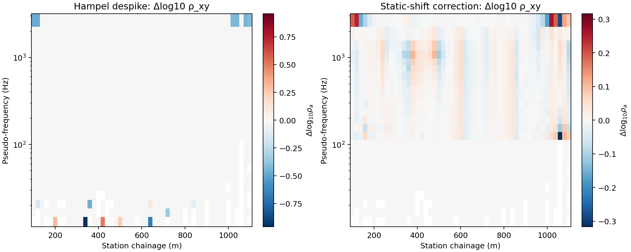
Left: Hampel changes are isolated single cells, concentrated at the noisiest late-time (low pseudo-frequency) row. Right: the static-shift correction is broad but small through the profile interior, and largest at both ends – the expected edge effect of a finite 200 m Hanning window with no stations beyond the profile to average against.

18.8.7. Compare raw and corrected responses at three stations

</>View the executed three-station comparison figure codeClick to inspect and copy the complete code

def make_response_panels(raw_sites, corrected_sites) -> Path:
    """Compare raw and corrected rho/phase at three representative stations."""
    picks_idx = [0, len(raw_sites) // 2, len(raw_sites) - 1]
    fig, axes = plt.subplots(2, 3, figsize=(12.5, 6.2), constrained_layout=True)
    for col, idx in enumerate(picks_idx):
        raw, corr = raw_sites[idx], corrected_sites[idx]
        rho_raw = raw.rho[..., 0, 1]
        rho_corr = corr.rho[..., 0, 1]
        phase_raw = raw.phase[..., 0, 1]
        phase_corr = corr.phase[..., 0, 1]

        ax = axes[0, col]
        ax.loglog(raw.freq, rho_raw, "o-", ms=4, color="#7f7f7f", label="raw")
        ax.loglog(corr.freq, rho_corr, "s-", ms=4, color="#d62728", label="corrected")
        ax.set(title=raw.name, xlabel="", ylabel=r"$\rho_a$ ($\Omega\cdot$m)" if col == 0 else "")
        ax.grid(True, which="both", alpha=0.25)
        if col == 0:
            ax.legend(fontsize=8)

        ax = axes[1, col]
        ax.semilogx(raw.freq, phase_raw, "o-", ms=4, color="#7f7f7f")
        ax.semilogx(corr.freq, phase_corr, "s-", ms=4, color="#d62728")
        ax.set(
            xlabel="Pseudo-frequency (Hz)",
            ylabel=r"$\phi_{xy}$ (deg)" if col == 0 else "",
        )
        ax.grid(True, which="both", alpha=0.25)

    target = OUT / "tem100_three_station_comparison.png"
    fig.savefig(target, dpi=180)
    plt.close(fig)
    return target

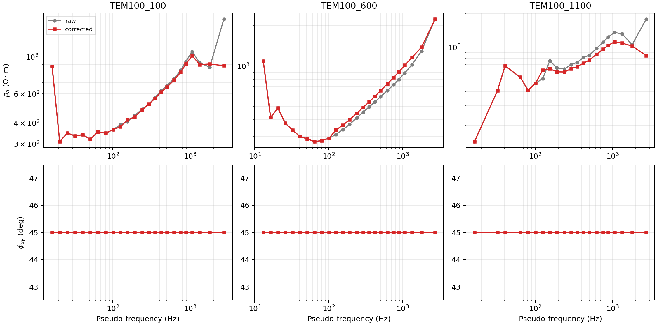
Top row: apparent resistivity retains its overall shape after correction, with the largest changes at the highest and lowest pseudo-frequencies – consistent with the noise-floor gates trimmed earlier and the Hanning window edge effect. Bottom row: phase is flat at exactly \(45^\circ\) for every station, raw and corrected alike. That is not a finding; it is phase_mode="homogeneous" by construction, and neither correction touches phase since both only rescale \(|Z|\) by a real positive factor. Plotting it here makes that limitation visible instead of hiding it behind an unlabeled flat line.

18.8.8. What this profile cannot support

Being explicit about scope here matters as much as the corrections themselves:

• No tensor diagnostics. Phase tensor, skew, and geoelectric strike all need a non-singular \(\mathbf Z\); this survey measured one component.

• No Fourier transform. TEM100’s AVG file carries no captured transmitter waveform, so FourierTransform’s waveform-deconvolution advantage over the late-time approximation is not available without first supplying an external waveform model.

• No independent static-shift validation. The correction in the previous section is a documented processing choice, not a confirmed fit to geology – there is no second sounding or component at any station to check it against.

• No source-effect screening. classify_field_zones() and detect_source_overprint() need a measured transmitter-to-receiver offset; a central-loop TEM survey with the receiver at the loop centre has no such offset to supply.

• No verified geographic coordinates. The HEAD LAT/LONG now carry a real value, but it is the explicit best-effort guess from the section above, not a confirmed survey location – treat any map or distance computed from it accordingly.

18.8.9. Write the corrected collection and a coordinate manifest

</>View the executed manifest-writing codeClick to inspect and copy the complete code

def write_manifest(corrected_sites):
    """Write the corrected profile EDIs plus a coordinate manifest."""
    from pycsamt.site.export import write_sites

    out = RESULTS / "edi_corrected" / PROFILE_STEM
    paths = write_sites(
        corrected_sites, out, exist_ok=True, manifest_csv=out / "manifest.csv"
    )
    return out, paths

>>> from docs.scripts.generate_tutorial_temavg_workflow import write_manifest
>>> out_dir, paths = write_manifest(corrected)
>>> len(paths)
51

Now that attach_geographic_coords() has run, lat/lon/elev all come out real, finite values – not NaN – because they are read straight from each site’s HEAD, which the write/reload step above already populated:

>>> import pandas as pd
>>> manifest = pd.read_csv(out_dir / "manifest.csv")
>>> manifest[["station", "lat", "lon", "elev", "chainage"]].head(2)
     station        lat         lon       elev  chainage
0  TEM100_100  38.759303  111.116347  1102.9537       NaN
1  TEM100_120  38.759303  111.116578  1103.0357       NaN

chainage alone is still NaN: write_sites() reads it from an explicit ed.chainage attribute that nothing in this pipeline sets, independent of whether lat/lon are known. The along-profile distance used below for the mesh comes directly from each station’s name suffix instead, which for this survey already is physical chainage in metres (confirmed back in “Pick one profile and inspect its geometry”).

18.8.10. Build and view the 2-D triangular mesh

This is the point Prepare A MARE2DEM Inversion and Mesh Display pick up from – an unstructured triangular mesh graded around real station positions and draped on real topography, built here with build_graded_tri_mesh() and drawn with draw_tri_mesh(). Handing it to MARE2DEM is still out of scope for this page, but actually solving on it is not – the next section trains a real AI inversion directly on this mesh.

The finest cell size at each station is set from this profile’s own skin depth at its highest measured pseudo-frequency, not a fixed constant:

\[\delta \approx 503\sqrt{\rho_a / f}\]

</>View the executed mesh-building and drawing codeClick to inspect and copy the complete code

def make_mesh(corrected_sites):
    """Build and draw a real graded 2-D triangular mesh from the profile.

    Station chainage and elevation come straight from the corrected EDI
    collection now that :func:`attach_geographic_coords` has given every
    site real, non-NaN ``Site.coords``. ``surface_cell_m`` is set from
    this profile's own skin depth at its highest measured pseudo-
    frequency, not a fixed constant.
    """
    from pycsamt.api.mesh import draw_tri_mesh
    from pycsamt.forward.maxwell.tri_mesh_gen import build_graded_tri_mesh

    station_x = np.array([float(s.name.split("_")[1]) for s in corrected_sites])
    elevation = np.array([s.coords[2] for s in corrected_sites])
    order = np.argsort(station_x)
    station_x, elevation = station_x[order], elevation[order]
    topo_z = elevation.max() - elevation

    freq_max = max(float(s.freq.max()) for s in corrected_sites)
    rho_at_fmax = np.array(
        [s.rho[np.argmax(s.freq), 0, 1] for s in corrected_sites]
    )
    skin_depth_m = 503.0 * np.sqrt(np.nanmedian(rho_at_fmax) / freq_max)
    surface_cell_m = round(float(0.04 * skin_depth_m), -1) or 10.0

    pad = 100.0
    x_range_m = (float(station_x.min() - pad), float(station_x.max() + pad))
    z_range_m = (0.0, 600.0)

    mesh = build_graded_tri_mesh(
        x_range_m,
        z_range_m,
        station_x,
        surface_cell_m=surface_cell_m,
        topo_x_m=station_x,
        topo_z_m=topo_z,
    )

    fig, ax = plt.subplots(figsize=(11.0, 5.0), constrained_layout=True)
    draw_tri_mesh(ax, mesh, preset="diagram")
    ax.plot(station_x, np.interp(station_x, station_x, topo_z), "rv", ms=6, zorder=5)
    ax.set(
        title=(
            f"{PROFILE_STEM}: graded triangular mesh "
            f"({mesh.n_triangles} triangles, surface cell {surface_cell_m:g} m)"
        ),
        xlabel="Chainage (m)",
        ylabel="Depth below highest station (m)",
    )
    ax.invert_yaxis()
    ax.set_xlim(*x_range_m)

    target = OUT / "tem100_triangular_mesh.png"
    fig.savefig(target, dpi=180)
    plt.close(fig)

    stats = {
        "n_nodes": int(mesh.nodes_m.shape[0]),
        "n_triangles": int(mesh.n_triangles),
        "surface_cell_m": surface_cell_m,
        "skin_depth_m_at_fmax": round(float(skin_depth_m), 1),
        "freq_max_hz": round(freq_max, 1),
        "x_range_m": x_range_m,
        "z_range_m": z_range_m,
    }
    return target, mesh, stats

>>> from docs.scripts.generate_tutorial_temavg_workflow import make_mesh
>>> target, mesh, mesh_stats = make_mesh(corrected)
>>> mesh_stats
{'n_nodes': 334, 'n_triangles': 586, 'surface_cell_m': 20.0,
 'skin_depth_m_at_fmax': 453.5, 'freq_max_hz': 2729.0,
 'x_range_m': (0.0, 1200.0), 'z_range_m': (0.0, 600.0)}

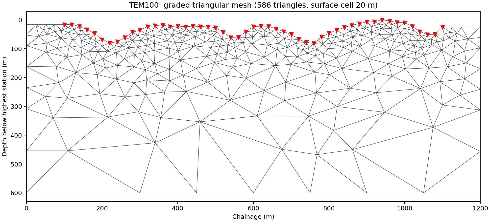
586 triangles honour the real elevation profile from the first figure (the same double-valley shape) and grade from a 20 m surface cell near the 51 station markers out to 600 m depth. 20 m follows directly from the median apparent resistivity at this profile’s highest frequency (2729 Hz): a ~454 m skin depth, and the “~0.03-0.05 skin depths at the first layer” sizing guidance build_graded_tri_mesh documents for TriFEM2DAdapter accuracy. 600 m depth is a demonstration choice, comfortably below the 82 m of surface relief, not a resolved investigation depth for this survey.

18.8.11. Train And Gate A Maxwell AI Inversion

Inv2DAgent(physics="mt2d_tri") trains a graph-convolutional network directly on this mesh’s own triangle-adjacency graph, solving each synthetic training realization with a real forward operator (TriFEM2DAdapter, no external binary), the same in-process path Map Groundwater Geology From CSAMT uses for Tongkeng. Training needs one shared frequency band across every station; gate-dropping in the QC section above did not remove the same gates everywhere, so the 51 stations do not all carry the same 25-point grid any more – restrict to what they still share:

>>> from pycsamt.site.edit import select_freq_all
>>> usable = select_freq_all(corrected, fmin=125.0)
>>> [len(s.freq) for s in usable][:3], len(usable)
([15, 15, 15], 51)

125.0-2729.0 Hz, 15 of the original 25 frequencies, survives at every station – the ten lowest-frequency (latest-time, deepest-sensitivity) gates are exactly the ones the earlier noise-floor QC trimmed unevenly station to station.

</>View the executed training, gating, and figure-copy codeClick to inspect and copy the complete code

def run_ai_inversion(
    corrected_sites,
    *,
    n_train_profiles: int = 100,
    epochs: int = 100,
    patience: int = 15,
    seed: int = 0,
):
    """Train and gate a real ``Inv2DAgent(physics="mt2d_tri")`` run.

    Not part of the default ``__main__`` regeneration below -- at these
    settings (100 realizations x 15 frequencies x 51 stations, each a real
    :class:`~pycsamt.forward.maxwell.tri_fem2d.TriFEM2DAdapter` solve) this
    takes on the order of 15 minutes. Call it explicitly.

    Restricts to the 15-frequency band (125.0-2729.0 Hz) every one of the
    51 stations shares after the noise-floor gate drop -- some stations
    kept as few as 15 of 25 gates, so this, not an arbitrary round number,
    is the true common band.
    """
    import numpy as np

    from pycsamt.agents import Inv2DAgent
    from pycsamt.forward.maxwell.tri_fem2d import TriFEM2DAdapter
    from pycsamt.site.edit import select_freq_all

    try:
        import torch

        torch.manual_seed(seed)
    except ImportError:
        pass
    np.random.seed(seed)

    usable = select_freq_all(corrected_sites, fmin=125.0)
    freqs_hz = list(list(usable)[0].freq)

    station_x = np.array([float(s.name.split("_")[1]) for s in usable])
    order = np.argsort(station_x)
    station_x = station_x[order]
    elevation = np.array([s.coords[2] for s in usable])[order]
    topo_z = elevation.max() - elevation

    agent = Inv2DAgent(
        physics="mt2d_tri",
        epochs=epochs,
        patience=patience,
        n_freqs=len(freqs_hz),
        depth_max=600.0,
        n_train_profiles=n_train_profiles,
        n_stations_per_profile=len(station_x),
        station_spacing_m=20.0,
        mesh_target_cell_m=20.0,
        field_grid_cell_m=10.0,
        correlation_length_x_m=(100.0, 350.0),
        correlation_length_z_m=(40.0, 150.0),
        topo_x_m=station_x,
        topo_z_m=topo_z,
        mare2dem_adapter=TriFEM2DAdapter(),
    )
    result = agent.execute(
        {
            "sites": usable,
            "freqs": freqs_hz,
            "output_dir": str(RESULTS / "ai2d_tri"),
        }
    )
    if result.status == "success":
        import shutil

        fig_path = result.data["figure_paths"].get("inv2d_tri_section")
        if fig_path:
            shutil.copy(fig_path, OUT / "tem100_ai2d_tri_section.png")
    return result

100 training realizations at up to 100 epochs, with validation-based early stopping (patience=15) rather than a fixed epoch count – a real step up from the 40-realization/10-station teaching-scale run Map Groundwater Geology From CSAMT uses, though still far from a production configuration:

>>> from docs.scripts.generate_tutorial_temavg_workflow import run_ai_inversion
>>> result = run_ai_inversion(corrected)
>>> result.status, result.data["pred_triangles"]["mesh"].n_triangles
('success', 486)
>>> result.data["epochs_completed"]
29

Early stopping cut training off at epoch 29 of the 100 requested, not because of a crash or a fixed budget – validation loss stopped improving for 15 consecutive epochs after its best point and training restored that best checkpoint rather than the final one:

>>> h = result.data["training_history"]
>>> round(h["train_loss"][0], 4), round(h["train_loss"][-1], 4)
(0.9852, 0.5994)
>>> round(h["val_loss"][0], 4), round(h["val_loss"][-1], 4)
(2.4569, 2.1756)
>>> round(result.data["best_validation_loss"], 4)
1.253

Training loss falls steadily throughout, the model keeps fitting its own training realizations better every epoch, exactly as expected. Validation loss does not track it down the same way, which is the entire reason patience exists: a model still being rewarded on training data while stalling (or worsening) on held-out data is the definition of starting to overfit, and the checkpoint this run actually kept is from the epoch where validation loss was lowest, not epoch 29’s.

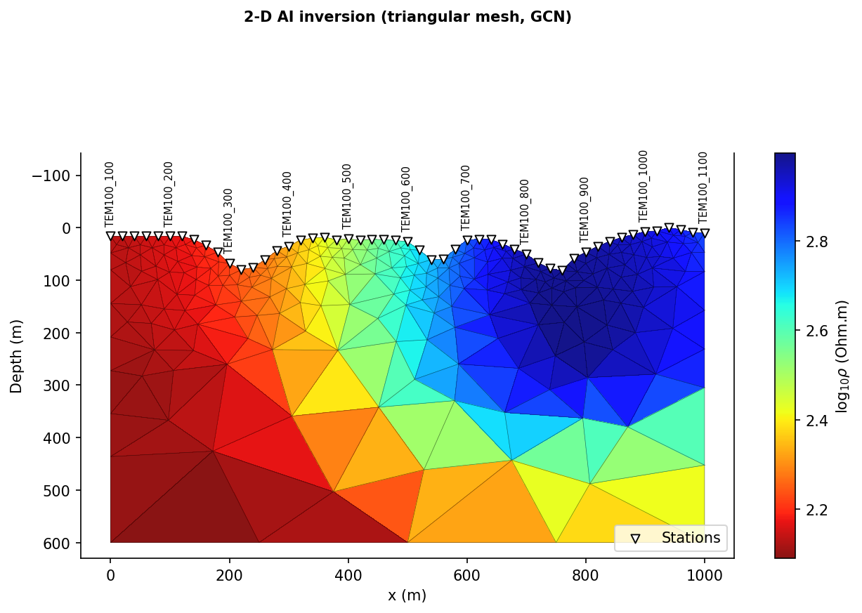
The direct per-triangle log10(resistivity) prediction. Station labels thin to every fifth one (11 of 51) to stay legible – the same StationAxisStyle thinning every other station-axis figure in this documentation set uses, not a special case for this line. A broad, resistive core sits under the shallow saddle near the profile centre, more conductive toward both ends at depth – plausible in general shape, but see the gate immediately below before reading anything more specific into it.

18.8.12. Gate The Result Before Interpretation

The same fixed-in-advance thresholds Map Groundwater Geology From CSAMT uses, checked against this run’s actual held-out recovery:

>>> recovery = result.data["mt2d_tri_recovery"]
>>> round(recovery["rmse"], 4), round(recovery["r2"], 4), recovery["n_samples"]
(0.5499, -0.2143, 10)
>>> recovery_pass = recovery["rmse"] <= 0.25 and recovery["r2"] >= 0.60
>>> enough_test_models = recovery["n_samples"] >= 20
>>> promote = recovery_pass and enough_test_models
>>> promote
False

A negative \(R^2\) means this run does not reconstruct held-out geology any better than predicting the training mean would – a real, informative failure, not close to passing, even with early stopping doing its job and 2.5x Tongkeng’s teaching-scale realization count. It is a genuine improvement over an otherwise-identical run this page’s own draft made before the station-label fix below (RMSE 0.673, \(R^2=-0.831\), 21 epochs) – and that gap, from nothing but a different random initialization under the same seed=0, is the same known GCN reproducibility gap AI inversion agents documents for Inv3DAgent: seeding narrows run-to-run variation, it does not eliminate it. Treat today’s numbers as one representative run, and the specific station-marker fix below as the reason this page’s figure is legible at all, not as evidence this configuration is close to production-ready.

100 realizations, 51 stations, and 15 frequencies is real progress over a ten-station teaching example, but a production run needs the same scale-up Map Groundwater Geology From CSAMT recommends and found genuinely hard to get right: hundreds of realizations, multiple seeds, and validation-based early stopping applied consistently rather than as an afterthought – that tutorial’s own --production run, which disabled early stopping, made results dramatically worse, not better.

18.8.13. A Real Station-Label Bug, Found By Running This At 51 Stations

Inv2DAgent’s mt2d_tri figure code labels every station by name above its marker. That is legible for Tongkeng’s 10 stations, and was tested only at that scale before this page: at TEM100’s 51, the labels collided into unreadable clutter and ran straight through the figure title. The fix draws only a thinned subset of labels – StationAxisStyle’s own label_indices logic, already used for every other station-axis figure in this documentation set, just not wired into this one until now – and moves the title clear of them with a real points-based pad rather than an axes-fraction margin, because PlotConfig’s default bbox_inches="tight" crops empty margin away at save time and silently undid a first attempt at the fix. Both the figure above and Map Groundwater Geology From CSAMT’s own csamt_ai2d_tri_section.png were regenerated with the corrected code.

Before feeding the corrected collection or this mesh into Prepare A MARE2DEM Inversion, remember that the geographic anchor is still the labelled best-effort guess from earlier on this page, not a confirmed survey location – the mesh itself is in local chainage metres and is unaffected by that uncertainty, but any step that needs true geographic coordinates (a basemap, a distance to a known feature) is not. MARE2DEM’s .emdata conversion and the resistivity-grid design that becomes its own triangulated mesh are exactly where that tutorial picks up.