6.2.6. Occam1D inversion

pycsamt.models.occam1d is pyCSAMT’s Occam1D engine: it builds native input files, runs the nonlinear smooth-model inversion, loads results, and produces review figures for one sounding at a time. Unlike Occam2D, which prepares files for an external Fortran executable, Occam1D’s forward model, analytic Jacobian, and Occam iteration are implemented natively in Python and NumPy – there is no external binary to compile or license for the default workflow, though Occam1DRunner can still drive one if a compiled Occam1D executable is available.

Every station is inverted independently. There is no mesh and no lateral coupling between soundings, so the regularization only penalizes roughness with depth at one station, following the same objective structure as any other Occam-family method (see objective function and (9) in Inversion):

(1)\[\mathrm{RMS} = \sqrt{\frac{1}{N}\sum_{i=1}^{N}\left(\frac{r_i}{\sigma_i}\right)^2},\]

the same RMS misfit used across pyCSAMT’s inversion engines, with \(r_i\) the residual at datum \(i\) and \(\sigma_i\) its assigned uncertainty. Occam1D searches, at each nonlinear iteration, for the smoothest layered-earth model whose predicted response drives this quantity toward a user-specified target.

6.2.6.1. When To Use Occam1D

Occam1D is the right tool when:

• soundings can be treated as independent 1-D layered earths – no profile geometry, no lateral mesh, no assumption that neighboring stations share structure;

• the deliverable is a fast, reproducible smooth inversion per station, suitable for a first pass over a whole survey before committing to a 2-D or 3-D engine;

• native file provenance (data, model, startup) still matters, e.g. for archiving or cross-checking against a reference Occam1D binary;

• batch throughput across many stations matters more than resolving 2-D or 3-D structure – see Batch inversion below.

It is not a substitute for Occam2D or ModEM when the target structure is genuinely two- or three-dimensional: a real lateral contact or dipping body will bias each independent 1-D model in a way no amount of per-station smoothness regularization can correct, because Occam1D has no mechanism to represent structure that only a neighboring station’s data constrains.

6.2.6.2. Package Map

Area	Main objects	Purpose
Configuration	Occam1DConfig	Mode, layer geometry, error floors, iteration controls, native filenames.
Input construction	Occam1DInputBuilder, Occam1DBatch	Build one station’s or a whole survey’s data/model/startup files from EDI or site sources.
Native data	Occam1DData, Occam1DModel, Occam1DStartup	Read/write the native sounding, layer geometry, and startup files.
Forward physics	Occam1DForwardModel	Isotropic layered-earth impedance recursion (analytic, optionally Numba-compiled).
Sensitivities	Occam1DJacobian	Analytic response derivatives, plus a central-difference reference path for verification.
Regularization	Occam1DRegularization, Occam1DSolverPolicy	Roughness penalty, linearized system assembly, ill-conditioning fallback policy.
Native inversion	Occam1DInversion	The nonlinear Occam loop itself: Lagrange multiplier search, model acceptance, convergence.
External execution	Occam1DRunner	Discover and launch an external Occam1D-compatible binary as an alternative to the native engine.
Results	Occam1DResult, Occam1DInversionResult, Occam1DRestart	Load a completed run’s iterations, response, and log; checkpoint and resume a native run.
Diagnostics	Occam1DResponse, Occam1DLog	Parse response residuals and convergence history from native files.
Plotting	PlotModel, PlotResponse, PlotConvergence, PlotSummary	Model, response-fit, convergence, and combined summary figures.
Validation	detect_file_type, scan_occam1d_directory, validate_occam1d_file	Recognize and check native data, model, and startup files.

6.2.6.3. Configuration

Occam1DConfig is the source-of-truth object for one station’s (or one batch’s) inversion setup. It groups four concerns: which response is extracted from the source data, how the layer geometry is discretized, how the nonlinear iteration is controlled, and what the native files are named.

>>> from pycsamt.models.occam1d import Occam1DConfig

>>> cfg = Occam1DConfig(
...     mode="determinant",
...     n_layers=30,
...     first_thickness=5.0,
...     depth_max=5000.0,
...     starting_resistivity=100.0,
...     target_misfit=1.5,
...     max_iterations=25,
... )
>>> cfg.layer_growth_factor
1.2008325637623543

>>> path = cfg.to_template("occam1d.yml")
>>> loaded = Occam1DConfig.from_file(path)
>>> loaded.mode, loaded.n_layers, loaded.depth_max, loaded.target_misfit
('determinant', 30, 5000.0, 1.5)

mode selects which response Occam1D fits: "xy"/"te" or "yx"/"tm" extract one polarization, while the default "determinant" fits the rotation-invariant determinant response \(Z_d=\sqrt{-Z_{xy}Z_{yx}}\), which is what pycsamt.models.occam1d.processing computes when no explicit resistivity/phase pair is supplied. n_layers, first_thickness, and depth_max define a geometrically growing layer stack: layer_growth_factor is derived, not stored, specifically so these three parameters cannot silently contradict each other. target_misfit and max_iterations bound the nonlinear search; error_floor_rho/ error_floor_phase (relative resistivity, absolute phase in degrees) set the minimum uncertainty assigned to any observation, which matters because Occam1D will otherwise happily overfit an observation whose reported error is implausibly small.

6.2.6.4. Build Input Files

The examples below use three real soundings from a public USGS magnetotelluric survey of the Gabbs Valley geothermal area, Nevada (Peacock et al., 2021, data/gv_data/README.md) – gv100, gv130, and gv163, spanning the low, middle, and high end of the 59-station numbering. Real field data (broadband, remote-reference processed, with some noisy long-period estimates) exercises the missing-observation handling and candidate rejection that a clean synthetic sounding would not.

>>> from pycsamt.models.occam1d import Occam1DBatch, Occam1DConfig
>>> from pycsamt.seg.edi import EDIFile

>>> stations = ["gv100", "gv130", "gv163"]
>>> sources = [
...     EDIFile(f"data/gv_data/gv_final_edi/{s}.edi") for s in stations
... ]
>>> config = Occam1DConfig(
...     mode="determinant",
...     n_layers=30,
...     first_thickness=5.0,
...     depth_max=5000.0,
...     starting_resistivity=100.0,
...     target_misfit=1.5,
...     max_iterations=25,
... )
>>> batch = Occam1DBatch(
...     sources, "occam1d-inversion", config=config
... ).build_all()
>>> batch.is_ready, len(batch.builders)
(True, 3)

Each station gets its own subdirectory (occam1d-inversion/gv100/, and so on), containing the three native files plus a JSON manifest recording the effective configuration and checksums:

>>> from pycsamt.models.occam1d import detect_file_type

>>> for name in ["Occam1DData", "Occam1DModel", "Startup"]:
...     print(name, detect_file_type(f"occam1d-inversion/gv100/{name}"))
Occam1DData Occam1DFileType.DATA
Occam1DModel Occam1DFileType.MODEL
Startup Occam1DFileType.STARTUP

gv100 keeps all 48 of its frequencies; gv130 and gv163 lose two of theirs. That is expected, not a bug to work around: real EDI files mark a missing transfer-function estimate with the format’s own EMPTY sentinel (1e32) rather than omitting the row, and the survey’s own metadata notes some long-period estimates are less robust. extract_sounding filters observations that are not finite and positive before a data row is ever written, so a station with a few unusable long-period estimates builds cleanly with a slightly shorter frequency list instead of propagating a sentinel value into the inversion.

6.2.6.5. Running The Inversion

Occam1DInversion runs the nonlinear Occam loop directly against the objects an Occam1DInputBuilder (or a batch’s builders) already prepared – no subprocess, no native file round-trip required to get started:

>>> from pycsamt.models.occam1d import Occam1DInversion

>>> builder = batch.builders[0]
>>> inversion = Occam1DInversion(
...     builder.data, builder.model,
...     config=builder.config, startup=builder.startup,
... )
>>> result = inversion.run()
>>> print(inversion.result_summary(result))
pyCSAMT native Occam1D inversion
  station       : gv100
  mode          : determinant
  frequencies   : 48
  observations  : 96
  layers        : 30
  status        : max_iterations
  iterations    : 25
  initial RMS   : 10.236448
  final RMS     : 1.6218702
  target RMS    : 1.5
  roughness     : 25.133911
  multiplier    : 0.05
  rejected      : 2247
  failed steps  : 0
  message       : The maximum iteration count was reached.

Each iteration evaluates the current model’s Lagrange multiplier against a small logarithmically spaced grid of trial factors (13 by default), solves the regularized linear system at every trial, scores every resulting candidate through the nonlinear forward model, and accepts the one that best trades off roughness against misfit – never a linearized estimate. The 2247 rejected candidates above are not a sign anything went wrong: at 13 trials per iteration across 25 iterations, most trials are supposed to lose to a better one every step, and every rejection is kept in result.rejected_candidates for exactly this kind of post-hoc check rather than discarded silently.

Behind inversion.run(), the same isotropic layered-earth recursion computes both the forward response and, simultaneously, its analytic derivative with respect to every layer’s log-resistivity. For angular frequency \(\omega\), layer resistivity \(\rho_j\), thickness \(h_j\), and vacuum permeability \(\mu_0\), define

(2)\[\gamma_j=\sqrt{i\omega\mu_0/\rho_j},\qquad \eta_j=\sqrt{i\omega\mu_0\rho_j},\qquad Z_j=\eta_j\,\frac{Z_{j+1}+\eta_j\tanh(\gamma_jh_j)} {\eta_j+Z_{j+1}\tanh(\gamma_jh_j)},\]

starting from the basement impedance \(Z_N=\eta_N\) and recursing upward to the surface impedance \(Z_1\). Apparent resistivity is \(|Z_1|^2/(\mu_0\omega)\) and phase is \(\arg(Z_1)\). This is the same recursion Forward Modelling uses for synthetic 1-D responses; Occam1D’s contribution is the outer nonlinear loop and regularization around it, not a separate physics implementation. When Numba is installed (an optional accelerator, not a hard dependency), this recursion runs as compiled per-frequency scalar code instead of NumPy calls on small arrays – roughly an order of magnitude faster per evaluation on real survey-sized soundings, with identical results either way, because the analytic Jacobian and every candidate evaluation call it once per trial multiplier.

For the determinant mode used above, the two off-diagonal impedance components combine as

(3)\[Z_d=\sqrt{-Z_{xy}Z_{yx}},\]

a rotation-invariant response that is less sensitive to a purely 2-D or 3-D distortion of any single component than xy or yx alone – part of why it is Occam1D’s default for field data where the true dimensionality is not yet known.

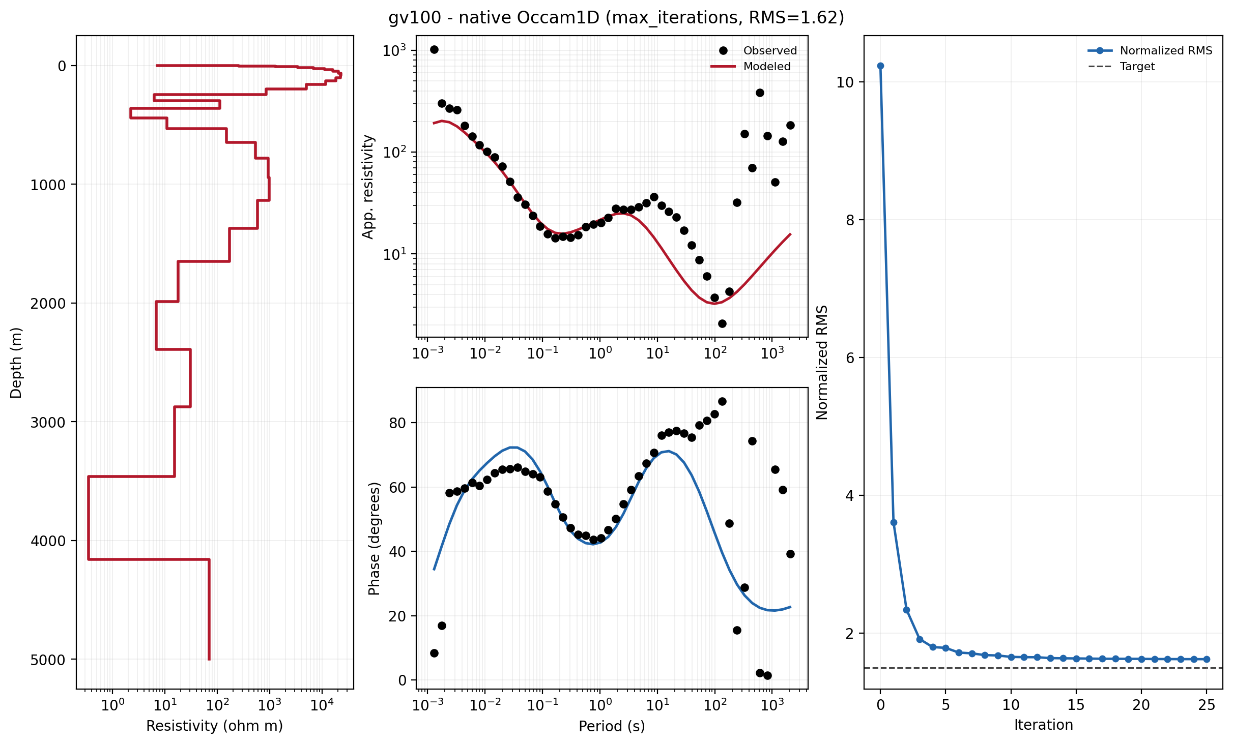
gv100’s combined summary figure: recovered resistivity-depth model (left), observed versus modeled apparent resistivity and phase (center), and RMS convergence history (right).

The model panel shows resistive near-surface layers giving way to a conductive zone around 300-600 m depth, then increasing resistivity with depth – broadly consistent with a shallow volcanic/sedimentary cover over more resistive basement, though a single 1-D sounding cannot by itself distinguish a genuine conductive layer from smoothed lateral structure. The fit panel shows the model tracking the observed curve well through the mid-band, with the largest departures at the shortest and longest periods, exactly where the survey metadata flags data quality as weaker; the convergence panel shows RMS dropping sharply in the first few iterations and then flattening well above the target of 1.5, consistent with real noise rather than a starting-model or convergence problem. This combined figure comes directly from save_main_images() — see Text and image products below – which is built from the same public PlotModel/PlotResponse/ PlotConvergence helpers used individually elsewhere in the package.

result is an immutable Occam1DInversionResult carrying the full accepted-model history (result.iterations), the starting and final models (result.initial/result.final, each an Occam1DIteration with .parameters in log10 resistivity, .rms, and .roughness), why the run stopped (result.convergence, an Occam1DConvergence value such as TARGET, MAX_ITERATIONS, or STAGNATED), and the full rejection/failure ledgers used above. Call restart() to checkpoint a run and continue it later with an absolute, not additive, iteration budget.

An external, separately compiled Occam1D-compatible binary remains an option through Occam1DRunner, which discovers an executable (explicit path, the run directory, or PATH) and launches it as a subprocess against the same native files:

>>> from pycsamt.models.occam1d import Occam1DRunner

>>> runner = Occam1DRunner(
...     "occam1d-inversion/gv100", binary_path="/opt/occam1d/Occam1D"
... )
>>> runner.run(target_misfit=1.5, max_iterations=25)

Note

Unlike Occam2D and ModEM, the pycsamt invert command line group does not currently cover Occam1D – --solver there accepts only occam2d and modem. Use the Python API shown on this page for Occam1D until CLI support is added.

6.2.6.6. Batch inversion

Because every station is independent, an entire survey can be built and inverted in two calls. Occam1DBatch.build_all prepares every station’s native files (shown above); invert_all then runs each one’s inversion to completion:

>>> outcome = batch.invert_all(n_jobs=1, export_text=False)
>>> for station, summary in sorted(outcome["results"].items()):
...     print(
...         f"{station}: status={summary['status']} "
...         f"iterations={summary['iterations']} "
...         f"final_rms={summary['final_rms']:.3f}"
...     )
gv100: status=max_iterations iterations=25 final_rms=1.622
gv130: status=max_iterations iterations=25 final_rms=3.755
gv163: status=max_iterations iterations=25 final_rms=2.523

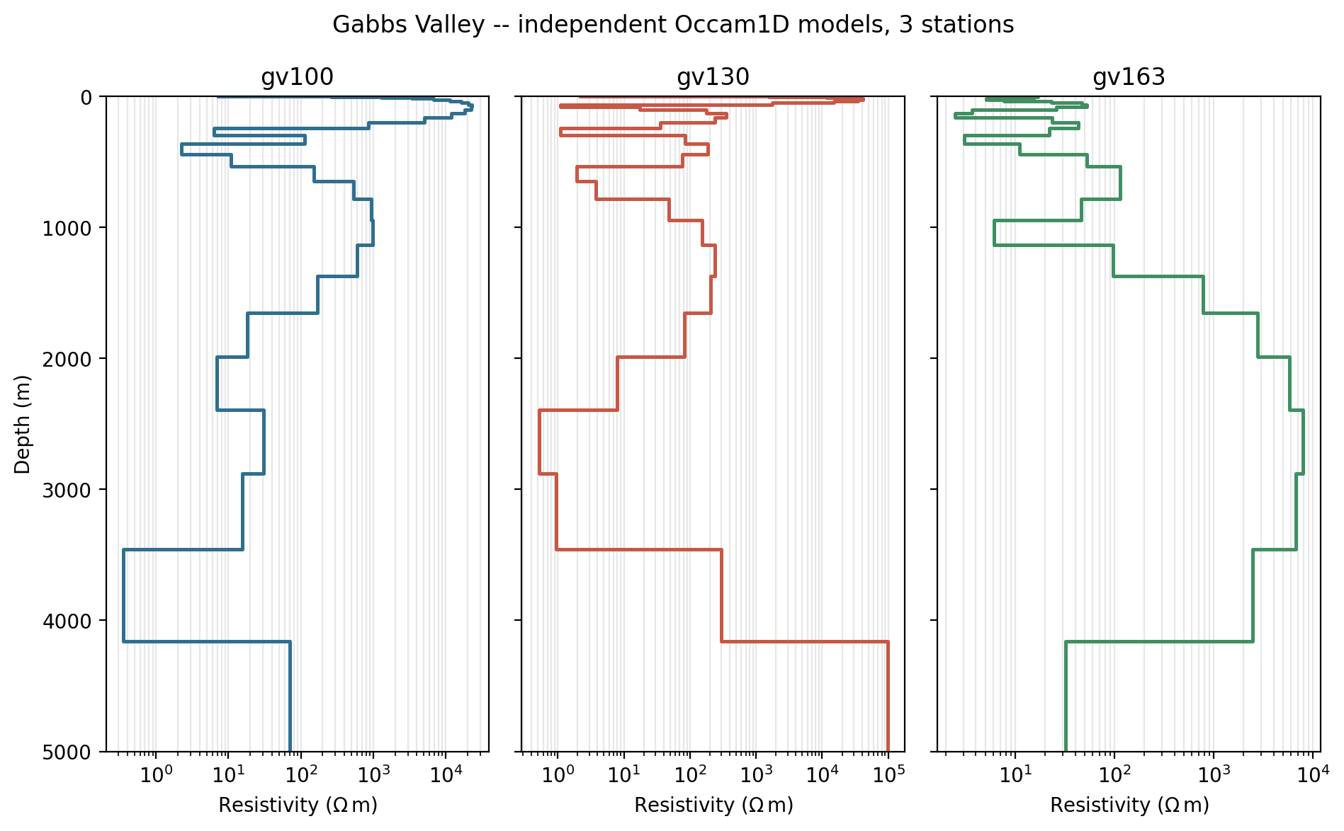
The three stations’ final models, one column per station on a single shared depth axis. Each panel is an independent inversion – Occam1D never shares information between stations – yet lining them up this way makes it easy to see that all three place a conductive zone within the top kilometre before trending resistive at depth, a first, informal check for whether the along-valley structure is at least broadly consistent before committing to a laterally coupled 2-D or 3-D inversion.

gv130 and gv163 converge to a visibly higher final RMS than gv100. That gap is a real, station-specific data-quality difference worth carrying into the interpretation, not a bug in the batch call – invert_all runs each station’s inversion with identical settings and reports whatever RMS that station’s own data actually supports.

Each station’s data, model, and startup are re-read from the files build_all already wrote rather than passed in memory, so invert_all(n_jobs=-1) can dispatch every station to a separate process through joblib without pickling problems. Stations are fully independent, so this scales close to linearly once a survey has comfortably more stations than worker processes; for a handful of stations, process start-up cost dominates and sequential execution (n_jobs=1, the default) is competitive. export_text/ export_images control whether each station also gets its usual CSV/JSON/PNG products written during the same call; both default to lighter settings suited to a first pass over a large survey.

joblib is an optional dependency (pip install pycsamt[perf]); without it, n_jobs other than 1 falls back to a sequential loop and a warning. Numba, also part of the perf extra, is the accelerator introduced above – both are soft dependencies specifically so a plain pip install pycsamt keeps working, only slower.

6.2.6.7. Text and image products

>>> text_paths = inversion.export_result("model-text")
>>> image_paths = inversion.save_main_images("model-image")
>>> sorted(text_paths)
['failures', 'iterations', 'metadata', 'model', 'rejected', 'response', 'summary']

The image export writes stable model, response, convergence, and combined summary PNG files (the last is what the figure above uses). Apparent resistivity is displayed in ohm metres, phase in degrees, frequency in hertz, and depth in metres. The model panel follows the pyCSAMT convention of positive depth downward and a filled downward station marker at the surface. The text export writes the same information as CSV/JSON, suitable for downstream scripting without re-parsing native files or re-running the inversion.

6.2.6.8. Common Mistakes

Treating rejected candidates as failures

A high rejected count in result_summary is routine: most of the 13 trial multipliers evaluated per iteration are expected to lose to a better one every step. Look at result.failed_iterations (candidates that could not be evaluated at all) for a genuine problem instead.

Reading a smooth conductive layer as a sharp boundary

Occam1D’s roughness penalty spreads structure with depth unless the data actively require a sharper transition. A gradational resistivity drop in the model panel does not imply a gradational geological contact.

Interpreting independent stations as a laterally coupled section

Nothing prevents plotting several stations’ 1-D models side by side (as above), but each one was inverted with zero knowledge of its neighbors. Apparent lateral continuity is a real observation worth checking, not a result the regularization enforced.

Leaving error floors at survey-wide defaults for noisy long-period data

error_floor_rho/error_floor_phase apply uniformly to every observation that passes the finite/positive filter. A station with markedly worse long-period estimates (like gv130/gv163 above) may need a higher floor, or an explicit freq_min/freq_max restriction, rather than letting the inversion chase noise.

6.2.6.9. Next Steps

• Occam2D – the 2-D counterpart, for genuinely laterally varying structure.

• Compiling the External Solvers – building an external solver, if Occam1DRunner’s binary path is preferred over the native engine.

• Inversion – the shared objective-function and regularization concepts behind every Occam-family engine in pyCSAMT.