11.27.2. Machine-Learning Quality Scoring

Quality-Control Confidence Scoring builds its confidence ratio from named, individually interpretable component scores – coverage, uncertainty, tensor shape, phase smoothness. That is a strength for auditability, but it also means every component is scored independently: nothing in the rule-based table notices that a station’s SNR, skew, and phase asymmetry are jointly unusual even when no single one crosses its own threshold. EMQCScorer adds that joint view. It keeps two hard, auditable rules from the rule-based world – a minimum SNR and a maximum Swift skew – and combines them with an isolation forest fitted on five per-(station, frequency) features:

• SNR – \(|\bar Z| / \sigma(Z)\), from the impedance error tensor when available, or from local spectral smoothness (a median-filter residual) otherwise;

• Swift skew – \(|\beta_\text{Swift}| = |(Z_{xx}+Z_{yy})/(Z_{xy}-Z_{yx})|\), the same regional-distortion diagnostic used throughout Phase Tensor And Impedance Tensor Tools;

• off-diagonal asymmetry – \(\log_{10}(|Z_{xy}|/|Z_{yx}|)\);

• phase of \(Z_{xy}\) and \(Z_{yx}\), in degrees.

Every observation that fails the hard SNR or skew rule is scored 0 outright. Surviving observations get a data-driven score in [0, 1] from the Isolation Forest’s decision function, min-max normalized across the batch and then combined with the rule outcome by geometric mean, so a rule pass cannot be overridden by the anomaly model but a rule pass alone does not guarantee a high score either.

11.27.2.1. Fitting and scoring

Load the bundled L18PLT line the same way Quality-Control Confidence Scoring does, then fit and score in two calls:

>>> from pathlib import Path
>>> from pycsamt.emtools import ensure_sites
>>> from pycsamt.ai.processing import EMQCScorer
>>> sites = ensure_sites(
...     Path("data/AMT/WILLY_DATA/L18PLT"),
...     recursive=True, on_dup="replace", strict=True,
... )
>>> scorer = EMQCScorer(random_state=0)
>>> scorer.fit(sites)
EMQCScorer(ml+rules)
>>> table = scorer.score_table(sites)
>>> table[["station", "freq", "score", "flag"]].head()
  station      freq     score  flag
0 18-001A  10400.0  0.940062     1
1 18-001A   8707.0  0.954844     1
2 18-001A   7289.0  0.949452     1
3 18-001A   6102.0  0.963360     1
4 18-001A   5108.0  0.982671     1

score_table mirrors station_confidence_table()’s row shape – station, freq, one column per feature, score, and a binary flag – so it can be filtered, merged, or exported the same way. On this line, 556 of the 1484 station-frequency cells (37%) fall below the default score_threshold=0.5:

>>> (table["flag"] == 0).sum(), len(table)
(556, 1484)

Warning

random_state=None by default, matching sklearn.ensemble.IsolationForest’s own default: every unseeded call to fit() trains a slightly different forest, and individual scores can shift by a few percent between runs. Pass an explicit random_state (as above) for a reproducible score table; the hard SNR/skew rules and their resulting flag values do not depend on the random state at all.

11.27.2.2. Reading the score chart

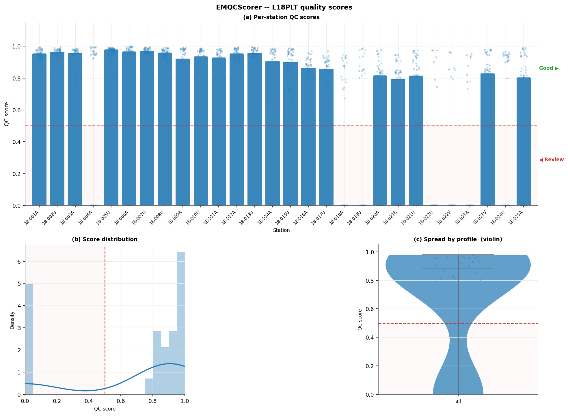
plot_qc_summary() on the L18PLT score table: (a) per-station bars are the median score over all 53 frequencies at that station, with individual per-frequency scores shown as translucent dots; (b) the pooled score distribution; (c) the same distribution as a violin.

Seven stations – 18-004A, 18-018A, 18-019U, 18-022U, 18-022V, 18-023A, 18-024U – sit at exactly zero in panel (a) even though their scattered per-frequency dots range up to 0.9 or higher. A median collapses to zero whenever more than half of a station’s frequencies are hard-flagged, and for these seven stations that is exactly what happens: more than half of their 53 frequencies carry a Swift skew above the skew_threshold=0.3 cutoff. That is a real electromagnetic signal, not scoring noise – these are the stations Learned Dimensionality Classification later classifies as predominantly 3-D – and it is a direct consequence of summarizing a per-frequency quantity with a single per-station number: always check the scatter, not just the bar, before excluding a station outright.

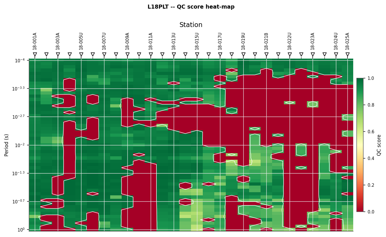
plot_qc_heatmap() – the same scores resolved by station and period, with the score=0.5 contour traced in white.

The heat-map makes the period dependence explicit: red regions cluster at the long-period (low-frequency) end for most stations, the classic signature of dead-band and cultural-noise contamination in AMT data, and the run of solid red across stations 18-018U through 18-023A at short period corresponds to the same skew-driven rejection seen in the summary bars.

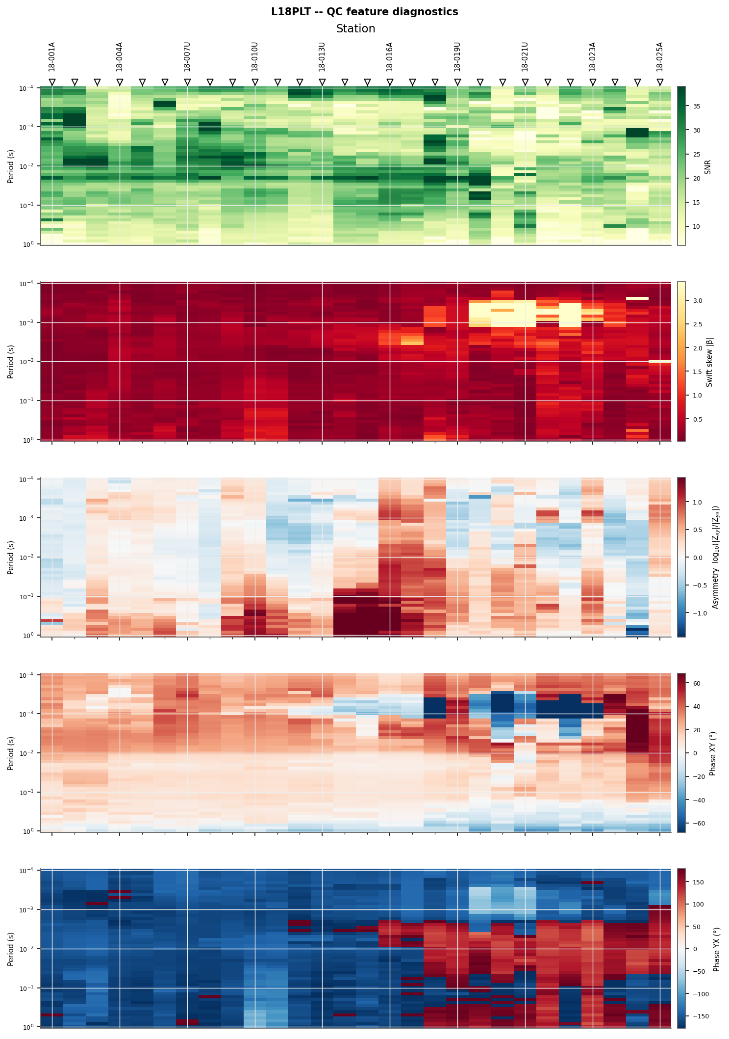
plot_qc_feature_heatmap() – one panel per input feature, letting you check why a region scored low rather than only that it did. The Swift-skew panel (second from top) shows the same stations lighting up pale yellow (skew well above the default 0.3 rule) that collapsed to zero in the summary bar chart.

11.27.2.3. Sites in, masked sites out

Everything above operates on a score_table() DataFrame. For everyday use, apply() follows the same sites-in / sites-out convention as Learned Spectral Denoising’s apply() and the rule-based notch_powerline(): pass a site collection, get one back with every hard-flagged station-frequency row masked (mode="mask", the default) or replaced by a linear interpolation from its nearest good neighbours (mode="interp") – the same two modes notch_powerline itself offers, reusing its own interpolation helper.

>>> masked_sites = scorer.apply(sites, mode="mask")
>>> len(list(masked_sites)) == len(list(sites))
True

Masking changes Z.z, not the station count: all 28 stations survive, but every flagged row across them now reads NaN in all four impedance components, ready to be dropped or down-weighted by whatever inversion input builder consumes masked_sites next.

>>> n_nan_before = 0  # sites: 0 masked rows anywhere
>>> n_nan_after = 556  # masked_sites: one NaN row per flagged cell
>>> n_nan_before, n_nan_after
(0, 556)

Warning

A whole frequency row is masked together – all four impedance components – even though only the off-diagonal components feed the score. This mirrors notch_powerline’s own convention: a hard-flagged frequency (failing the SNR or skew rule) is treated as unreliable across the board, not selectively for the components that happened to trigger the rule.

11.27.2.4. Parameters

contamination (default 0.05) is the Isolation Forest’s expected outlier fraction and controls how aggressively it separates the “normal” region of feature space; raise it if you expect a noisier survey, lower it for a clean, well-instrumented one. snr_threshold (default 3.0) and skew_threshold (default 0.3) are the two hard rules described above – tightening either one increases the number of stations forced to a median of zero the way panel (a) shows. score_threshold (default 0.5) only affects the binary flag column and the plotted “Good” / “Review” split; it does not change the underlying score. Set use_ml=False to disable the Isolation Forest entirely and fall back to the two hard rules alone (scores are then strictly 0 or 1) – useful as a sanity baseline before trusting the combined score, or when scikit-learn is unavailable.

Full parameter and return-value documentation is in the API reference: EMQCScorer and plot_qc_scores(), plot_qc_heatmap(), plot_qc_feature_heatmap(), plot_qc_score_distribution(), plot_qc_score_spread(), and plot_qc_summary(). Every plotting function accepts a plain ndarray, a {profile: ndarray} dict, or the score_table() DataFrame directly, and every station-axis function accepts a StationTickConfig for fine control over tick spacing on long profiles.

</>View the complete EMQCScorer example sourceClick to inspect and copy the complete code

def run_qc(sites, save_dir: Path) -> None:
    print("\n=== EMQCScorer ===")
    scorer = EMQCScorer(random_state=0)
    scorer.fit(sites)
    table = scorer.score_table(sites)
    print(f"  rows: {len(table)}")
    print(f"  stations: {table['station'].nunique()}")
    print(f"  flagged bad: {(table['flag'] == 0).sum()} "
          f"/ {len(table)}")
    print(table[["station", "freq", "score", "flag"]].head(5)
          .to_string(index=False))

    fig = plot_qc_summary(
        table, score_threshold=0.5,
        suptitle="EMQCScorer -- L18PLT quality scores",
    )
    _save(fig, save_dir, "qc_summary.png")

    ax = plot_qc_heatmap(table, title="L18PLT -- QC score heat-map")
    _save(ax.figure, save_dir, "qc_heatmap.png")

    fig = plot_qc_feature_heatmap(
        table, title="L18PLT -- QC feature diagnostics"
    )
    _save(fig, save_dir, "qc_feature_heatmap.png")

Point load_l18() at your own EDI folder to adapt this script