6.3.5. Domain-gap and noise simulation

A geological prior generator plus a verified forward solver, as described in Correlated geological priors and either 2-D Maxwell training-data generation or 3-D Maxwell training-data generation, produces clean, noiseless responses. Field data is never that well behaved. pycsamt.ai.domain_gap exists to close some of that domain gap deliberately, by turning a clean SurveyData into one with realistic error floor, heteroscedastic noise, static shift, galvanic distortion, missing stations or frequencies, and undetected outliers — instead of hoping that a generic noise term covers what a real survey actually looks like. Every corruption function below operates on the canonical SurveyData contract alone, with no notion of how many spatial dimensions produced it, so the same simulator applies unchanged whether the clean input came from a 2-D section or a 3-D volume — domain-gap simulation and forward-solver dimensionality are orthogonal concerns.

6.3.5.1. Two families of corruption

simulator splits its corruption functions into two families that behave differently on purpose. Systematic effects multiply the true impedance by a per-station real matrix and leave the shape of the declared error to scale with it. apply_static_shift() draws a station’s shift factor log-normally,

(1)\[c_s = 10^{\,X_s}, \qquad X_s \sim \mathcal N(0, \sigma_{\log_{10}}^2),\]

so that \(\sigma_{\log_{10}}\) (static_shift_log10_sigma) is a decade-scale spread rather than a linear one, matching how static shift is normally reported:

>>> import numpy as np
>>> from pycsamt.ai.data.contracts import SurveyData
>>> from pycsamt.ai.domain_gap.simulator import apply_static_shift

>>> z = np.ones((3, 2, 2), dtype=complex) * (100 + 100j)
>>> survey = SurveyData(
...     z, [10.0, 1.0], ["A", "B", "C"], ["xy", "yx"],
...     [[0, 0], [1, 0], [2, 0]],
... )
>>> shifted, info = apply_static_shift(
...     survey, log10_sigma=0.15, rng=np.random.default_rng(2),
...     return_info=True,
... )
>>> np.round(info["static_shift_factor"], 4)
array([1.0675, 0.8348, 0.867 ])

apply_galvanic_distortion() follows the same idea with a full Groom-Bailey-style real 2x2 matrix per station,

(2)\[\begin{split}D_s = g_s\,R(\theta_s) \begin{bmatrix} 1+e_s & s_s \\ s_s & 1-e_s \end{bmatrix},\end{split}\]

combining a gain \(g_s\) (log-normal, like the static-shift factor), a rotation \(R(\theta_s)\) by a twist angle \(\theta_s\), a shear \(s_s\), and an anisotropy \(e_s\) — each independently normal with its own configured standard deviation — and applies \(D_s\) to every frequency of that station’s impedance at once. Systematic effects change the signal; they do not, by themselves, say anything about how much to trust it.

The matrix operation is exact only when the complete xx, xy, yx, yy tensor is present. If a clean 2-D or 3-D dataset retains only xy and yx, the implementation treats the missing diagonal terms as zero before applying \(D_s\). That is a documented augmentation approximation, not a reconstruction of the unobserved tensor. Full-tensor 3-D forward responses should therefore remain full tensor through distortion simulation whenever the training feature contract can consume them.

Random effects are the opposite: they update impedance_error and the validity mask directly, so a corrupted survey’s declared uncertainty stays honest about what was actually injected. add_heteroscedastic_noise() adds complex Gaussian noise per (station, frequency) pair scaled by a relative level drawn uniformly from a configured range, and combines it with any pre-existing declared error in quadrature rather than overwriting it. For an observation \(Z_{sfc}\), the implemented draw and propagated one-sigma error are

(3)\[\begin{split}\begin{aligned} \widetilde Z_{sfc} &= Z_{sfc} + \alpha_{sf}|Z_{sfc}| \frac{\epsilon_R + i\epsilon_I}{\sqrt{2}}, &\alpha_{sf} &\sim \mathcal U(\alpha_{\min},\alpha_{\max}),\\ \epsilon_R,\epsilon_I &\sim \mathcal N(0,1), &\widetilde\sigma_{sfc} &= \sqrt{\sigma_{sfc}^2+(\alpha_{sf}|Z_{sfc}|)^2}. \end{aligned}\end{split}\]

The \(1/\sqrt{2}\) factor makes \(\mathbb E[|\widetilde Z-Z|^2]=\alpha_{sf}^2|Z|^2\); without it, the requested complex-noise variance would silently be doubled. apply_error_floor() clamps the declared error to a minimum fraction of \(|Z|\).

(4)\[\sigma'_{sfc}=\max\!\left(\widetilde\sigma_{sfc}, \eta|\widetilde Z_{sfc}|\right),\]

where \(\eta\) is error_floor_fraction. The floor changes the declared uncertainty, not the impedance itself; it must therefore not be interpreted as a mechanism that shifts the mean response. apply_dropout() marks whole stations, whole frequencies, or individual observations missing by setting impedance to NaN, which SurveyData construction then turns into the authoritative validity mask automatically — no separate bookkeeping needed. inject_outliers() does the opposite of dropout: it perturbs a fraction of otherwise valid observations by a large factor without invalidating them, simulating a bad reading that quality control failed to flag — exactly the case a robust downstream inverter has to tolerate, not just detect.

The three dropout probabilities are independent draws before their masks are combined. Consequently, a cell survives with probability

(5)\[P(\text{valid after dropout}) = (1-p_s)(1-p_f)(1-p_o),\]

provided it was valid on input. Here \(p_s\), \(p_f\), and \(p_o\) are station, frequency, and observation dropout rates. Their sum is therefore not the expected missing fraction.

6.3.5.2. Composing one reproducible pass

A real survey was not corrupted by one effect at a time, and neither should a training example be. apply_corruption_suite() runs every step above in one fixed, physically motivated order — static shift and distortion first, then noise, error floor, dropout, outliers, and coordinate/elevation perturbation. A single seed spawns an independent child generator per step, so adding a new step later does not change what every earlier step draws. It returns both the corrupted survey and a CorruptionRecord of exactly what was sampled, not just what was requested. Four named severities in SEVERITY_PRESETS turn a whole parameter block into one word:

Preset	Noise level	Static shift \(\sigma_{\log_{10}}\)	Station dropout	Outlier rate
clean	0	0	0	0
in_distribution	1-3%	0.05	0	0
severe	5-15%	0.15	5%	2%
held_out_corruption	10-25%	0.30	15%	8%

clean is the required control set every Loss functions for scientific inversion/ Recovery, residual, and OOD diagnostics comparison needs a baseline from; held_out_corruption is deliberately outside the range a model should have been trained to expect, for out-of-distribution checks.

The record makes a generated sample auditable rather than merely repeatable. It stores the complete configuration, its SHA-256 hash, the parent seed, the preset name, and compact summaries of the concrete draws:

>>> import numpy as np
>>> from pycsamt.ai.data.contracts import SurveyData
>>> from pycsamt.ai.domain_gap import apply_corruption_suite

>>> survey = SurveyData(
...     np.ones((8, 10, 1), dtype=complex) * (100 + 100j),
...     np.logspace(2, -1, 10),
...     [f"S{i}" for i in range(8)], ["xy"],
...     np.column_stack([np.arange(8) * 100, np.zeros(8)]),
... )
>>> corrupted, record = apply_corruption_suite(
...     survey, severity="severe", seed=7
... )
>>> corrupted.n_valid, survey.n_valid
(70, 80)
>>> record.severity
'severe'
>>> sorted(record.sampled)
['distortion_twist_deg_mean', 'dropped_fraction',
 'dropped_frequency_count', 'dropped_station_count', 'n_outliers',
 'static_shift_factor_mean']
>>> record.to_dict()["config_hash"][:12]
'c91ce027d0f0'

The seed reproduces the draw; the hash proves which parameter block was used. Both belong in the run manifest described in AI inversion reporting.

Coordinate and elevation perturbation need special care in a genuine 3-D workflow. perturb_coordinates() changes the reported receiver geometry but deliberately leaves impedance unchanged. It models location uncertainty in graph construction or preprocessing; it is not a second Maxwell solve at the displaced receivers, does not alter the solver mesh, and does not introduce topography into the physics. If the intended experiment is sensitivity of impedance to receiver position or terrain, rebuild the Maxwell problem and run the chosen forward adapter at each perturbed geometry instead.

One clean geological realization may produce several corruption variants, but those variants are not independent earth models. Assign each one a lineage key such as (dataset_id, realization_id) and split on that parent key before selecting clean, in_distribution, severe, or held_out_corruption variants. Otherwise a clean response can enter training while its noisy copy enters validation or test, giving an optimistically biased result. Store the child corruption seed and CorruptionRecord beside the immutable parent ID; the configuration hash alone identifies the recipe, not the parent realization.

6.3.5.3. Fitting corruption from a real survey

Guessed corruption ranges are still a guess. The more useful path is fitting them from a real survey’s own quality-control diagnostics. survey_data_from_sites() bridges anything ensure_sites() accepts into a canonical SurveyData, converting impedance from the EDI-native [mV/km]/[nT] convention z stores to the SI convention SurveyData declares — a real unit mismatch found and fixed while building this bridge, confirmed against rho’s own field-convention apparent resistivity to floating-point precision. From there, fit_corruption_config() reads noise and dropout directly from the survey’s declared impedance_error and coverage, while fit_distortion_priors_from_sites() calls the existing pycsamt.emtools.gb.groom_bailey_table() and pycsamt.emtools.ss.estimate_ss_ama() diagnostics directly on the sites to get an empirical static-shift and distortion spread — the one part of this package that genuinely depends on a specific survey rather than on literature defaults:

>>> from pycsamt.emtools._core import ensure_sites
>>> from pycsamt.ai.domain_gap import (
...     survey_data_from_sites,
...     fit_corruption_config,
...     fit_distortion_priors_from_sites,
... )

>>> sites = ensure_sites(
...     "data/AMT/WILLY_data/L18PLT", recursive=True, verbose=0
... )
>>> field = survey_data_from_sites(sites, recursive=False, verbose=0)
>>> field.shape
(28, 53, 4)

>>> config = fit_corruption_config(field)
>>> tuple(round(v, 4) for v in config.noise_level_range)
(0.0509, 0.1582)
>>> round(config.error_floor_fraction, 4)
0.0297

The fitted noise range (5-16% relative) and error floor (about 3% of \(|Z|\)) come entirely from L18’s own declared errors, not from a default — a survey with tighter QC would fit a narrower range without anyone having to retune a preset by hand.

These fitted values describe the observation process represented by L18; they are not evidence that a synthetic geological prior covers L18’s earth responses. They may be applied to clean MT1D, MT2D, MT3D, or ModEM-generated surveys because all use the same SurveyData contract, while the forward backend and its mesh provenance remain attached to the clean parent realization.

More precisely, the fitter uses the finite ratios \(r=\sigma_Z/|Z|\): the 25th and 75th percentiles define the noise range, while the 5th percentile defines the floor. Missing fractions by station, frequency, and observation supply the corresponding dropout rates. severity_scale multiplies those estimates before rates are clipped to \([0,1]\); it is a controlled stress multiplier, not a statistically fitted confidence bound. Static shift and distortion priors must still be fitted from sites separately because they require the Groom–Bailey and AMA diagnostics, not only the canonical error tensor.

6.3.5.4. Comparing simulated and field distributions

Fitting a corruption config is not, by itself, evidence that it closes the domain gap. report computes that evidence directly: per-feature summary statistics and a two-sample Kolmogorov–Smirnov statistic between a simulated and a field survey, on log_impedance_magnitude, phase_deg, and error_to_magnitude_ratio — features derived from the shared SurveyData contract so the comparison never depends on how either survey was produced. The real M3 workflow applies a field-fitted config to a clean synthetic survey, not back onto the field survey itself, so the comparison actually tests whether a generic geological prior looks like the target survey:

For empirical cumulative distribution functions \(F_n\) and \(G_m\), the reported statistic is

(6)\[D_{n,m}=\sup_x |F_n(x)-G_m(x)|.\]

\(D=0\) means the empirical distributions coincide; larger values identify a stronger marginal mismatch. The accompanying p-value tests an equal-distribution null hypothesis, but it is sample-size dependent and is not an engineering acceptance threshold. Define tolerances for the KS statistic, mean difference, and standard-deviation ratio before looking at the result, and compare frequency bands and component sets that are scientifically commensurate.

>>> from pycsamt.ai.geology import GeologyGrid
>>> from pycsamt.ai.training.dataset2d import (
...     Maxwell2DDatasetConfig,
...     generate_2d_maxwell_dataset,
... )
>>> from pycsamt.ai.domain_gap import (
...     apply_corruption_suite,
...     compare_survey_distributions,
... )

>>> grid = GeologyGrid.regular_2d(nx=10, nz=8, dx_m=300, dz_m=150)
>>> ds_config = Maxwell2DDatasetConfig(
...     dataset_id="willy-like-clean",
...     grid=grid,
...     correlation_length_x_m=(600.0, 1200.0),
...     correlation_length_z_m=(200.0, 400.0),
...     frequencies_hz=np.logspace(0, 4, 20),
...     station_x_m=list(np.linspace(500.0, 2500.0, 10)),
...     n_realizations=1,
...     seed=1,
...     log_resistivity_mean=2.0,
...     log_resistivity_std=0.4,
...     validation_fraction=0.0,
...     test_fraction=0.0,
... )
>>> dataset = generate_2d_maxwell_dataset(ds_config)
>>> clean_synthetic = dataset.samples[0].survey

>>> corrupted, record = apply_corruption_suite(
...     clean_synthetic, config, seed=3
... )
>>> report = compare_survey_distributions(corrupted, field)
>>> magnitude = report.comparisons["log_impedance_magnitude"]
>>> round(magnitude.ks_statistic, 4), round(magnitude.mean_difference, 4)
(0.1376, 0.0445)
>>> phase = report.comparisons["phase_deg"]
>>> round(phase.ks_statistic, 4), round(phase.mean_difference, 2)
(0.2908, -13.13)

The small magnitude mean difference says that these two examples happen to share a similar central magnitude scale. It does not show that the fitted noise or error floor caused the match: equation (4) changes uncertainty only, and the noise in equation (3) is zero-mean. The magnitude KS statistic of 0.14 still exposes differences in distribution shape. The phase comparison is the more honest result: a KS statistic of 0.29 and a 13-degree mean offset show that a generic correlated-field prior with only kilometre-scale correlation lengths does not reproduce L18’s real phase behaviour, which reflects genuine 2-D and 3-D structure this small demonstration grid was never built to represent. That gap is exactly what Correlated geological priors and Forward Modelling’s survey-specific tuning — not the noise model — would need to close; report is what makes that distinction visible instead of hiding it behind one aggregate “looks about right.”

The same distinction is visible in a smaller deterministic diagnostic. The upper panels below show how systematic shifts create station-wise vertical bands, outliers form isolated extreme cells, and dropout cuts white holes through an otherwise smooth response. In the empirical CDFs below them, the magnitude curves nearly overlap (\(D=0.002\)) while a six-degree phase displacement produces \(D=0.303\). A survey can therefore look suitably messy and still have the wrong physics in one feature.

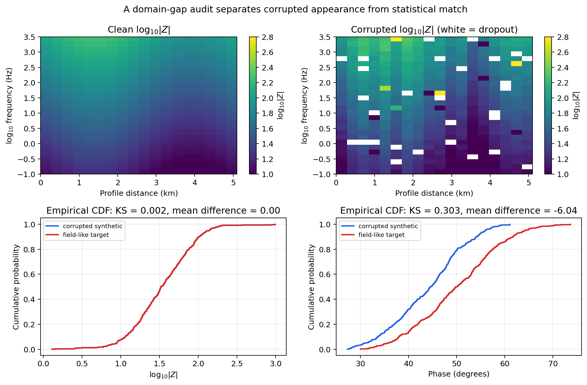
A reproducible domain-gap diagnostic generated with apply_corruption_suite() and compare_survey_distributions().

6.3.5.5. Accounting for every station, not just corruption

A different, related question — is this survey internally coherent enough to trust at all, station by station — is audit_survey()’s job, covered in full in Accounting for every station, not just the aggregate. It lives in this package for the same reason the functions above do: it depends on the pandas-based dimensionality and distortion diagnostics pycsamt.ai.data deliberately excludes.