
7.3. Borehole logs#
Interpretation workflow already shows the everyday path for
a Borehole: load one from CSV, give it a
profile position, and hand it to
ModelCalibrator as a ground-truth constraint.
This page does not repeat that walkthrough. It covers what a
Borehole and its Interval
records actually offer beyond that one call – querying a log
directly, building one without a CSV file, and reading LAS 2.0 well
logs, which Interpretation workflow mentions but does not
demonstrate.
Note
This lightweight class represents one vertical log at a profile-relative
x coordinate. For a universal, spatial, multi-hole exchange document
with CRS, deviation surveys, multiple log families, structures, and PCSF
association, use PCBH — Common Borehole Format.
7.3.1. Querying a log directly#
A Interval is a leaf value object
in the sense introduced in Package concepts: bottom must exceed
top, checked once in __post_init__ (see Package concepts for
why editing one after construction via clone()/update() does
not re-check this). thickness and contains() are the two
things every other method on this page is built from:
>>> from pycsamt.geology import Borehole, Interval
>>> intervals = [
...     Interval(top=0.0, bottom=8.0, lithology="lateritic soil", resistivity=450.0),
...     Interval(top=8.0, bottom=31.0, lithology="clayey sand", resistivity=42.0),
...     Interval(top=31.0, bottom=67.0, lithology="weathered granite", resistivity=185.0),
...     Interval(top=67.0, bottom=120.0, lithology="fresh granite", resistivity=3200.0),
... ]
>>> intervals[0].thickness
8.0
>>> intervals[0].contains(4.0), intervals[0].contains(8.0)
(True, False)
A Borehole collects them and is just as
usable built directly from a list as it is loaded from a file –
useful for a log entered by hand, generated from a database query, or
assembled in a test:
>>> bh = Borehole("BH01", x=500.0, intervals=intervals, collar_elevation=238.4)
>>> bh
Borehole('BH01', x=500.0 m, 4 intervals, depth=120.0 m)
>>> bh.min_depth, bh.max_depth
(0.0, 120.0)
contains() is a half-open interval (top <= z < bottom), so
every depth belongs to exactly one interval except the log’s own
lower bound. interval_at_depth(), tres_at_depth(), and
lithology_at_depth() look a single depth up against it, returning
None – not raising – outside the logged range:
>>> bh.interval_at_depth(50.0)
Interval(top=31.0, bottom=67.0, lithology='weathered granite', resistivity=185.0)
>>> bh.tres_at_depth(50.0)
185.0
>>> bh.lithology_at_depth(50.0)
'weathered granite'
>>> bh.tres_at_depth(500.0) is None
True
tres_column() vectorizes the same lookup over an array of depths
– exactly what ModelCalibrator uses
internally to compare a model column against this log, cell by cell,
before blending:
>>> import numpy as np
>>> z = np.array([4.0, 20.0, 50.0, 100.0, 150.0])
>>> bh.tres_column(z)
array([ 450.,   42.,  185., 3200.,   nan])
The last depth (150 m) is below max_depth (120 m) and comes back
nan rather than extrapolated – a calibrator or any other consumer
of tres_column() should treat nan as “no ground truth here”,
not as zero resistivity. Drawing the log as a resistivity-versus-depth
step curve and marking exactly where those five z values land
makes the boundary behaviour easy to see at a glance:
View the tres_column sampling figure source codeClick to inspect and copy the complete code
 1def make_borehole_tres_sampling() -> None:
 2    """Write the ``tres_column()`` sampling figure for BH01.
 3
 4    Draws BH01's log as a resistivity-vs-depth step curve and marks
 5    where ``tres_column(z)`` samples it for a hypothetical model's
 6    depth cells, distinguishing a found value from ``nan`` below
 7    ``max_depth`` -- what a calibrator sees when it reads this log
 8    cell by cell.
 9    """
10    bh01 = _make_bh01()
11    z = np.array([4.0, 20.0, 50.0, 100.0, 150.0])
12    tres = bh01.tres_column(z)
13
14    fig, ax = plt.subplots(figsize=(7, 5))
15
16    for iv in bh01.intervals:
17        ax.hlines(iv.resistivity, iv.top, iv.bottom, color="#2E4053", linewidth=3, zorder=2)
18    for i in range(len(bh01.intervals) - 1):
19        top = bh01.intervals[i + 1].top
20        r0 = bh01.intervals[i].resistivity
21        r1 = bh01.intervals[i + 1].resistivity
22        ax.vlines(top, min(r0, r1), max(r0, r1), color="#2E4053", linewidth=1.2,
23                  linestyle="--", zorder=2)
24        ax.vlines(top, 1, min(r0, r1), color="0.75", linewidth=0.8, zorder=1, linestyle=":")
25
26    found = np.isfinite(tres)
27    ax.scatter(z[found], tres[found], color="#C0392B", zorder=4, s=50,
28               label="tres_column() -- found")
29    ax.scatter(z[~found], np.full((~found).sum(), 1.5), color="#C0392B",
30               zorder=4, s=60, marker="x", linewidth=2,
31               label="tres_column() -- nan (below max_depth)")
32
33    for zi, ti in zip(z, tres):
34        label = f"z={zi:.0f}\n{'nan' if not np.isfinite(ti) else f'{ti:.0f}'}"
35        y = 1.5 if not np.isfinite(ti) else ti
36        ax.annotate(label, (zi, y), textcoords="offset points", xytext=(0, 10),
37                    ha="center", fontsize=8)
38
39    ax.axvline(bh01.max_depth, color="0.4", linestyle="-.", linewidth=1)
40    ax.text(bh01.max_depth + 2, 2000, f"max_depth={bh01.max_depth:.0f} m",
41            fontsize=8, color="0.3")
42
43    ax.set_yscale("log")
44    ax.set_ylim(1, 9000)
45    ax.set_xlim(-5, 160)
46    ax.set_xlabel("Depth z (m)")
47    ax.set_ylabel(r"Resistivity ($\Omega\,\mathrm{m}$, log scale)")
48    ax.set_title("BH01.tres_column(z) sampled against the logged intervals", pad=14)
49    ax.grid(alpha=0.25)
50    ax.legend(loc="upper left", fontsize=8)
51
52    fig.tight_layout()
53    fig.savefig(IMAGES / "borehole_tres_sampling.png", dpi=200, bbox_inches="tight")
54    plt.close(fig)
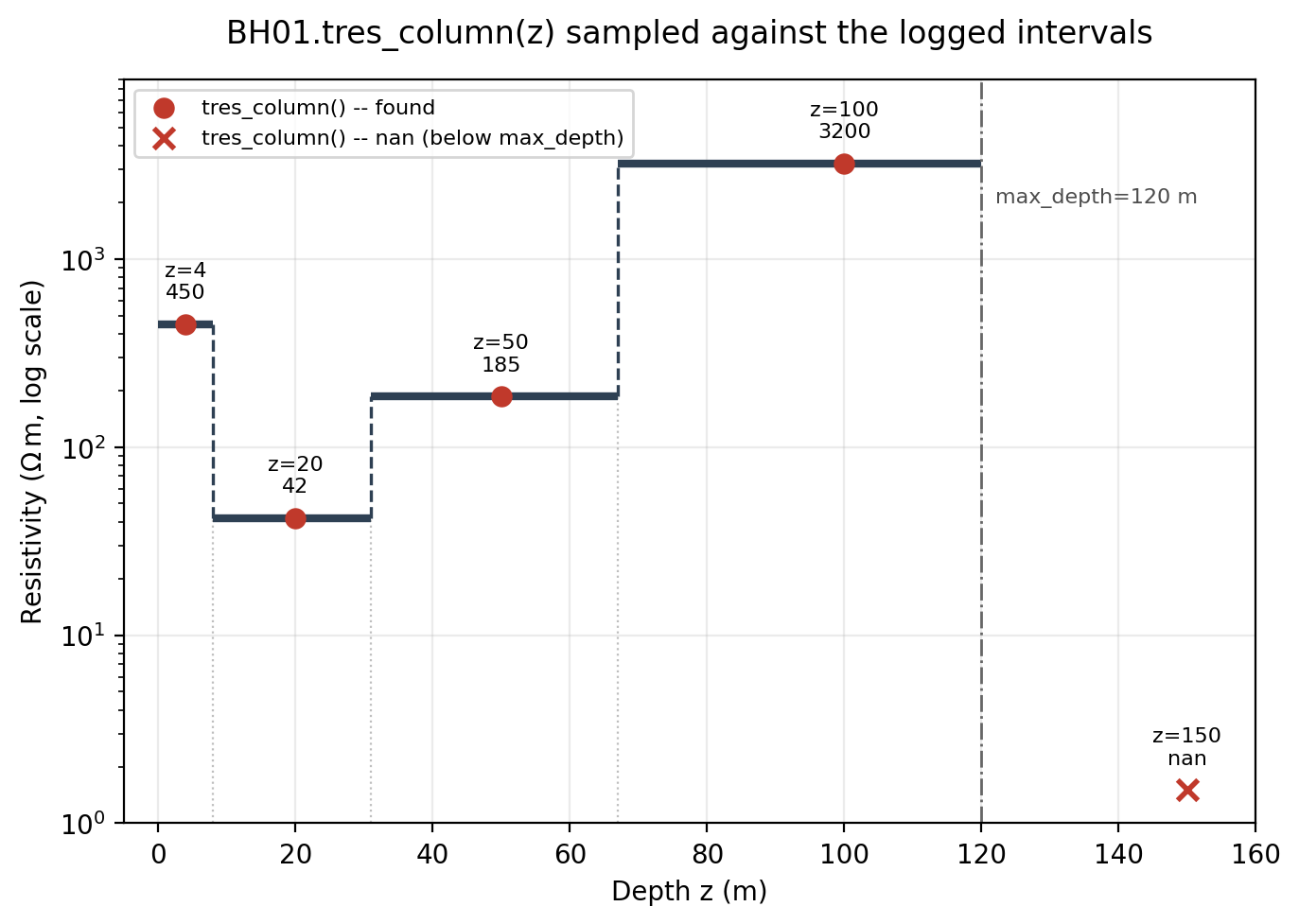
Each dot is one tres_column() result at the requested depth; the
x marker at z=150 sits below max_depth and comes back
nan rather than a value read off the deepest interval.#
7.3.2. Boreholes across a profile#
A single log is only half the picture – what makes a
Borehole useful in pycsamt is having several
of them positioned along the same profile as independent ground-truth
control points. Adding a shallow log and a deeper one alongside BH01,
each with its own x:
>>> bh03 = Borehole("BH03", x=150.0, intervals=[
...     Interval(top=0.0, bottom=6.0, lithology="topsoil", resistivity=300.0),
...     Interval(top=6.0, bottom=35.0, lithology="saprolite", resistivity=120.0),
...     Interval(top=35.0, bottom=60.0, lithology="fresh basement", resistivity=8000.0),
... ])
>>> bh04 = Borehole("BH04", x=900.0, intervals=[
...     Interval(top=0.0, bottom=15.0, lithology="alluvium", resistivity=30.0),
...     Interval(top=15.0, bottom=45.0, lithology="aquifer sand", resistivity=90.0),
...     Interval(top=45.0, bottom=60.0, lithology="clay aquitard", resistivity=8.0),
...     Interval(top=60.0, bottom=90.0, lithology="bedrock", resistivity=4000.0),
... ])
>>> [bh03.x, bh.x, bh04.x]
[150.0, 500.0, 900.0]
There is nothing linking these three Borehole objects to each
other beyond sharing the same profile coordinate system – no shared
container class is required to plot or reason about them together,
since x alone is enough to place each one correctly:
View the profile-position figure source codeClick to inspect and copy the complete code
 1def make_borehole_profile_positions() -> None:
 2    """Write the three-borehole profile-position figure.
 3
 4    Three independently constructed boreholes (BH01, plus a shallow
 5    BH03 and a deeper BH04), drawn as vertical log strips at their own
 6    ``x`` -- the picture a set of ground-truth control points along a
 7    survey line actually looks like before any of them reach a
 8    calibrator.
 9    """
10    bh01 = _make_bh01()
11    bh03 = Borehole("BH03", x=150.0, intervals=[
12        Interval(top=0.0, bottom=6.0, lithology="topsoil", resistivity=300.0),
13        Interval(top=6.0, bottom=35.0, lithology="saprolite", resistivity=120.0),
14        Interval(top=35.0, bottom=60.0, lithology="fresh basement", resistivity=8000.0),
15    ])
16    bh04 = Borehole("BH04", x=900.0, intervals=[
17        Interval(top=0.0, bottom=15.0, lithology="alluvium", resistivity=30.0),
18        Interval(top=15.0, bottom=45.0, lithology="aquifer sand", resistivity=90.0),
19        Interval(top=45.0, bottom=60.0, lithology="clay aquitard", resistivity=8.0),
20        Interval(top=60.0, bottom=90.0, lithology="bedrock", resistivity=4000.0),
21    ])
22    boreholes = [bh03, bh01, bh04]
23
24    all_liths: list[str] = []
25    for bh in boreholes:
26        for iv in bh.intervals:
27            if iv.lithology not in all_liths:
28                all_liths.append(iv.lithology)
29    palette = cm.get_cmap("tab20").colors
30    lith_color = {name: palette[i % len(palette)] for i, name in enumerate(all_liths)}
31
32    fig, ax = plt.subplots(figsize=(8, 6))
33    width = 60.0
34    for bh in boreholes:
35        for iv in bh.intervals:
36            ax.fill_betweenx(
37                [iv.top, iv.bottom], bh.x - width / 2, bh.x + width / 2,
38                color=lith_color[iv.lithology], edgecolor="0.25", linewidth=0.6,
39            )
40        ax.text(
41            bh.x, -3.0, f"{bh.name}\nx={bh.x:.0f} m",
42            ha="center", va="bottom", fontsize=9, fontweight="bold",
43        )
44
45    max_depth = max(bh.max_depth for bh in boreholes)
46    ax.set_xlim(0, 1050)
47    ax.set_ylim(max_depth + 5, -12)
48    ax.set_xlabel("Profile position x (m)")
49    ax.set_ylabel("Depth (m)")
50    ax.set_title("Three boreholes positioned along one survey profile")
51    ax.grid(axis="both", alpha=0.25)
52
53    handles = [plt.Rectangle((0, 0), 1, 1, color=lith_color[name]) for name in all_liths]
54    ax.legend(
55        handles, all_liths, loc="upper center", bbox_to_anchor=(0.5, -0.12),
56        ncol=4, fontsize=8, frameon=False,
57    )
58
59    fig.tight_layout()
60    fig.savefig(
61        IMAGES / "borehole_profile_positions.png", dpi=200, bbox_inches="tight"
62    )
63    plt.close(fig)
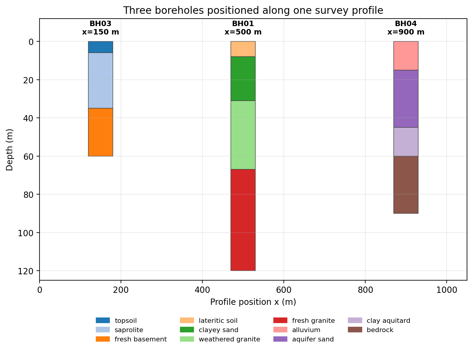
BH03, BH01, and BH04 drawn at their real x positions along a
shared profile axis – the same spatial layout
ModelCalibrator sees when it blends
several boreholes into one resistivity model in
Interpretation workflow. Depth increases downward in every
strip; only the profile position changes between them.#
7.3.3. Reading a LAS 2.0 log#
from_las() reads the industry-standard
LAS 2.0 well-log ASCII format directly, converting a continuous depth
curve into discrete intervals by grouping consecutive samples that
share the same lithology code. A minimal LAS 2.0 file has a well
section, a curve section naming each column by its mnemonic, and an
ASCII data section:
~VERSION INFORMATION
VERS.   2.0 : CWLS LOG ASCII STANDARD - VERSION 2.0
WRAP.    NO : ONE LINE PER DEPTH STEP
~WELL INFORMATION
WELL.        BH02 : WELL NAME
NULL.    -9999.25 : NULL VALUE
~CURVE INFORMATION
DEPT.M       : DEPTH
RESD.OHMM    : DEEP RESISTIVITY
LITH.        : LITHOLOGY CODE
~ASCII
0.0     450.0   1
2.0     430.0   1
4.0     410.0   1
6.0      60.0   2
8.0      45.0   2
10.0     40.0   2
12.0    190.0   3
14.0    180.0   3
Reading it groups the eight 2 m samples into three intervals, one per run of a constant lithology code, with the interval’s resistivity set to the mean of the samples inside it:
>>> bh_las = Borehole.from_las("BH02.las", x=750.0)
>>> bh_las
Borehole('BH02', x=750.0 m, 3 intervals, depth=16.0 m)
>>> for iv in bh_las.intervals:
...     print(iv)
Interval(top=0.0, bottom=6.0, lithology='1', resistivity=430.0)
Interval(top=6.0, bottom=12.0, lithology='2', resistivity=48.333333333333336)
Interval(top=12.0, bottom=16.0, lithology='3', resistivity=185.0)
The default curve mnemonics are DEPT for depth and RESD for
resistivity; override them with depth_curve/resistivity_curve
for a file that names them differently. lithology above is the
literal LAS code ('1', '2', '3') rather than a rock name –
LAS 2.0 has no standard mapping from a numeric lithology code to a
name, so from_las does not invent one. Remap the codes to names
your project recognises before comparing this log’s lithology
field against a RockDatabase classification;
comparing the resistivity values directly, as
ModelCalibrator does, needs no such mapping.
Pass lithology_curve=None for a file with no lithology curve at
all – every interval then gets the same generic label instead.
Plotting both logs side by side as a classic resistivity-versus-depth
track makes the difference between the two construction paths
concrete: BH01’s four hand-specified intervals on the left, BH02’s
eight raw 2 m samples collapsing into three from_las-grouped
intervals on the right.
View the log-comparison figure source codeClick to inspect and copy the complete code
 1def make_borehole_log_comparison() -> None:
 2    """Write the two-panel BH01/BH02 well-log figure.
 3
 4    Left panel: BH01, drawn as a classic resistivity-vs-depth log track
 5    colored by lithology. Right panel: BH02, showing the raw 2 m samples
 6    alongside the three intervals ``from_las`` grouped them into.
 7    """
 8    bh01 = _make_bh01()
 9    bh02 = _make_bh02()
10
11    fig, axes = plt.subplots(1, 2, figsize=(9, 6))
12
13    ax = axes[0]
14    for iv, color in zip(bh01.intervals, _BH01_COLORS):
15        ax.fill_betweenx(
16            [iv.top, iv.bottom], 0, iv.resistivity,
17            color=color, edgecolor="0.2", linewidth=0.7,
18        )
19        ax.text(
20            iv.resistivity * 1.15, (iv.top + iv.bottom) / 2,
21            f"{iv.lithology}\n{iv.resistivity:.0f} Ohm.m",
22            va="center", fontsize=8,
23        )
24    ax.set_xscale("log")
25    ax.set_xlim(1, 2e4)
26    ax.set_ylim(bh01.max_depth, 0.0)
27    ax.set_xlabel(r"Resistivity ($\Omega\,\mathrm{m}$, log scale)")
28    ax.set_ylabel("Depth (m)")
29    ax.set_title(f"{bh01.name} -- from_csv / direct construction")
30    ax.grid(axis="x", which="both", alpha=0.3)
31
32    ax = axes[1]
33    ax.scatter(
34        _BH02_RAW_RESD, _BH02_RAW_DEPTHS,
35        s=30, color="0.15", zorder=3, label="raw 2 m samples",
36        edgecolor="white", linewidth=0.6,
37    )
38    for iv, color in zip(bh02.intervals, _BH02_COLORS):
39        ax.fill_betweenx(
40            [iv.top, iv.bottom], 0, iv.resistivity,
41            color=color, alpha=0.55, edgecolor="0.2", linewidth=0.7,
42        )
43        ax.text(
44            iv.resistivity * 1.15, (iv.top + iv.bottom) / 2,
45            f"code {iv.lithology}\nmean {iv.resistivity:.0f}",
46            va="center", fontsize=8,
47        )
48    ax.set_xscale("log")
49    ax.set_xlim(1, 2e3)
50    ax.set_ylim(bh02.max_depth, 0.0)
51    ax.set_xlabel(r"Resistivity ($\Omega\,\mathrm{m}$, log scale)")
52    ax.set_title(f"{bh02.name} -- from_las grouping")
53    ax.grid(axis="x", which="both", alpha=0.3)
54    ax.legend(loc="lower right", fontsize=8)
55
56    fig.tight_layout()
57    fig.savefig(IMAGES / "borehole_log_comparison.png", dpi=200, bbox_inches="tight")
58    plt.close(fig)
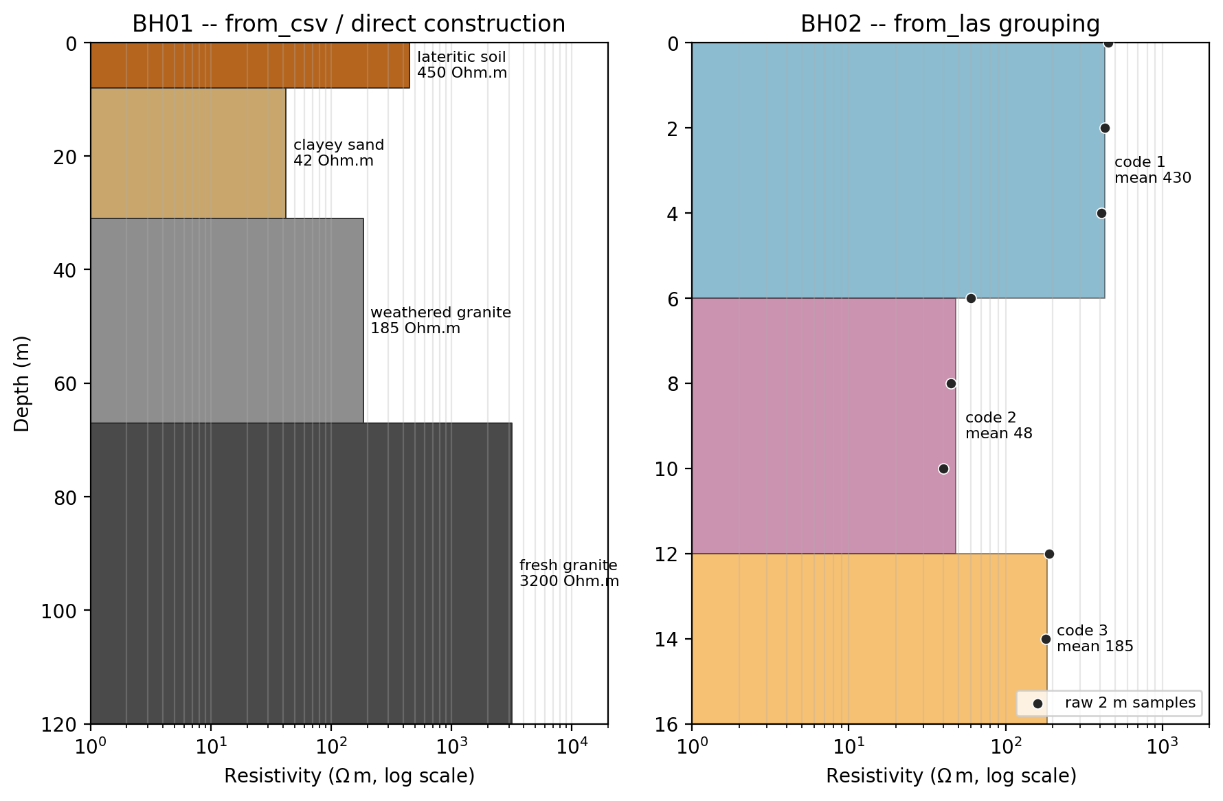
BH01 (left), colored by lithology from the intervals built directly above. BH02 (right), with the eight raw LAS samples as dots and the three grouped intervals as shaded bands – the boundary between the blue and pink bands falls exactly where the lithology code changes from 1 to 2, between the samples at 4 m and 6 m.#
7.3.4. Serializing a log#
to_dataframe() (requires pandas) and to_dict() both
flatten a Borehole for export or storage; unlike most classes in
this package, Borehole writes both by hand rather than relying on
to_dict(), so that the
thickness column below is always present without being stored
redundantly on every Interval:
>>> bh_small = Borehole("BH01", x=500.0, intervals=intervals[:2])
>>> bh_small.to_dataframe()
   top  bottom  thickness       lithology  resistivity
0  0.0     8.0        8.0  lateritic soil        450.0
1  8.0    31.0       23.0     clayey sand         42.0
7.3.5. Where to go next#
Interpretation workflow covers loading a log from CSV and
using it as a ModelCalibrator constraint end
to end. Rock resistivity database and Structural measurements cover the other two
data families in this package.