6.3.8. 3-D Maxwell training-data generation#

Solver-neutral Maxwell contracts solves one Maxwell problem at a time, in whichever dimension a backend supports. Training a network on genuinely 3-D structure needs many such volumes, each converted into the same shape every later stage agrees on. generate_3d_maxwell_dataset() is that bridge for the third dimension: it draws a correlated 3-D resistivity volume from geology for each realization, solves it with the research-only, small-grid MT3DAdapter through solve_batch(), and packages every realization that converges into a Maxwell3DDataset with a realization-level train/validation/test split and a DatasetManifest. A realization whose solve does not converge is recorded and excluded, never silently included – the same contract 2-D Maxwell training-data generation already enforces for two dimensions.

The module exists to give Inv3DAgent’s physics="mt3d" mode (AI inversion agents) something better than tiled independent 1-D columns to train on. Genuine 3-D Maxwell training means every synthetic example is a spatially varying three-dimensional conductivity volume whose response comes from one coupled solve, not from stitching per-station 1-D results together and letting a graph network’s spatial smoothing paper over the seams afterward. Architecture roadmap tracks this as M8’s research slice – wired end to end, but explicitly not yet the milestone’s production backend, which still targets the external, verified ModEm3DAdapter once its remaining open items close.

As with the 2-D generator, this one is best read as four linked contracts rather than one large function call: a geological volume defines the target, a padded solver mesh and receiver layout define the forward problem, canonical SurveyData defines the response axes, and the split plus manifest define which accepted realizations may be used for each statistical role. The third dimension changes the middle two contracts the most – a uniform mesh that stays affordable at production scale in 2-D is not affordable here, which is most of what makes this module more than a coordinate relabeling of 2-D Maxwell training-data generation.

6.3.8.1. Configuring a 3-D dataset#

A Maxwell3DDatasetConfig fixes everything that must stay identical across realizations: the shared (z, y, x) GeologyGrid, three correlation-length ranges instead of two – horizontal in x, horizontal in y, and vertical in z – the shared frequency grid, receiver (x, y) positions rather than a single x array, and a root Random seed from which every realization’s correlation, field, and solver seeds derive deterministically, following the same named-process hierarchy (9) describes for the geological prior:

>>> from pycsamt.ai.geology import GeologyGrid
>>> from pycsamt.ai.training.dataset3d import (
...     Maxwell3DDatasetConfig,
...     generate_3d_maxwell_dataset,
... )

>>> grid = GeologyGrid.regular_3d(
...     nx=4, ny=4, nz=6, dx_m=200, dy_m=200, dz_m=100
... )
>>> config = Maxwell3DDatasetConfig(
...     dataset_id="demo-3d-v1",
...     grid=grid,
...     correlation_length_x_m=(400.0, 800.0),
...     correlation_length_y_m=(400.0, 800.0),
...     correlation_length_z_m=(100.0, 200.0),
...     frequencies_hz=[50.0, 20.0],
...     station_xy_m=[[400.0, 400.0], [600.0, 600.0]],
...     n_realizations=2,
...     seed=0,
...     validation_fraction=0.0,
...     test_fraction=0.0,
... )
>>> config.components
('zxy', 'zyx')
>>> config.grid.shape, config.station_xy_m.shape
((6, 4, 4), (2, 2))
>>> config.to_dict()["schema_version"]
1

>>> dataset = generate_3d_maxwell_dataset(config)
>>> len(dataset.samples), dataset.rejected
(2, ())

station_xy_m is an (n_stations, 2) array rather than 2-D Maxwell training-data generation’s single station_x_m axis, because a 3-D receiver no longer sits on the one profile line a 2-D section implies – it needs both horizontal coordinates. Every accepted realization comes back as a Maxwell3DSample pairing the true resistivity volume (the training target) with its simulated SurveyData response (the training input) and the solver’s own mesh size and residual:

>>> sample = dataset.samples[0]
>>> sample.survey.shape
(2, 2, 2)
>>> sample.resistivity_ohm_m.shape
(6, 4, 4)
>>> sample.mesh_cells, round(sample.relative_residual, 6)
(3584, 0.0)
>>> f"{sample.relative_residual:.3e}"
'2.004e-19'

The geological grid holds 96 cells (\(6\times4\times4\)); the solver mesh that produced this sample already needs 3,584, even at documentation scale with two stations and two frequencies. That thirty-seven-fold gap is the entire subject of the next section, not an incidental detail – it is why a 2-D-style uniform mesh does not carry over to three dimensions.

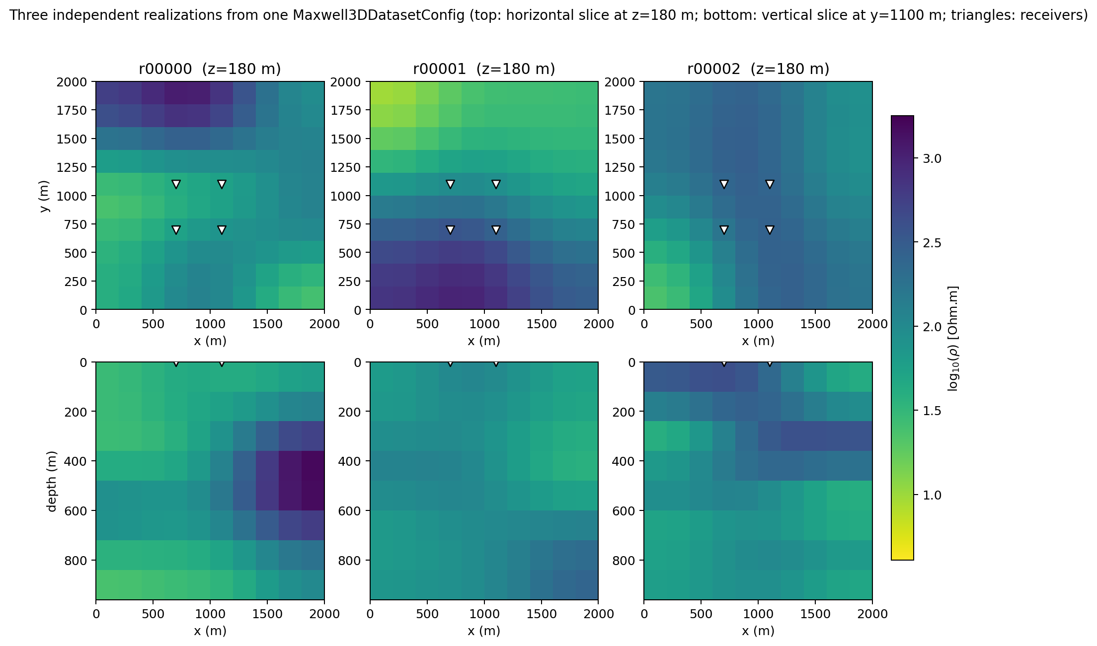
Three independent 3-D resistivity volumes shown as a horizontal slice and a vertical slice per realization, from one shared Maxwell3DDatasetConfig. — Three realizations from one `Maxwell3DDatasetConfig`. Top row: a horizontal slice at fixed depth, one column per realization, with the four receivers (white triangles) at their shared `(x, y)` positions. Bottom row: a vertical slice through the same volume at fixed `y`. All six panels share one color scale.#

Reading a column top-to-bottom is the point of this figure. In the leftmost realization the horizontal slice shows a resistive body in the upper-left quadrant, and the vertical slice below it shows a different structure – a resistive zone appearing only below roughly 300 m near the right edge, not a downward continuation of the shallow body above it. A field generated by tiling independent 1-D columns could never produce this: every column would be internally layered but identical in cross-section to its neighbours except where the tiling itself changes. Here, resistivity genuinely depends on all three coordinates at once, which is the property Genuine 3-D Maxwell training refers to and the reason the middle realization’s shallow slice (pale, resistive throughout) looks nothing like its own deeper slice (uniformly mid-range) a few panels below.

6.3.8.2. A padded mesh, not a uniform one#

2-D Maxwell training-data generation affords a uniform lateral mesh because 2-D solver cell count scales with the square of resolution. In three dimensions it scales with the cube:

(1)#\[N_{\text{cells}}\ \approx\ \frac{L_x}{h_x}\cdot\frac{L_y}{h_y}\cdot\frac{L_z}{h_z},\]

where each \(L\) is the mesh’s padded extent along one axis and each \(h\) is its cell width there. A uniform mesh fine enough to resolve a few-hundred-metre structure and extensive enough to reach several skin depths in three independent directions at once is rarely affordable within Maxwell3DDatasetConfig.max_mesh_cells. This module instead builds a padded, non-uniform mesh: a core region at the geological grid’s own native resolution – an exact, no-resample match to the model there – surrounded by cells that grow geometrically outward in x/y and downward in z until the padded extent reaches mesh_safety_factor times the deepest relevant skin depth. Far-field cells stay cheap without ever coarsening the region that matters.

This is the same strategy mt3d’s own calibrated benchmark mesh uses, and for the same reason it was added there in the first place: an earlier, uniform-only version of that solver failed its layered-earth benchmark by 30-45%, which first looked like a boundary-condition defect but turned out to be a mesh limitation – a uniform mesh could not reach several skin depths of padding and resolve a few-hundred-metre layer interface within the same cell budget, because refining resolution on a small uniform domain does not add padding, and adding padding on a coarse uniform mesh does not add resolution. Generalizing the solver’s discrete curl operators to non-uniform cell widths broke that trade-off; see mt3d’s module docstring for the full diagnosis. This module’s own mesh construction exists so that fix has somewhere to be used from training-data code, not just from a hand-built benchmark.

6.3.8.3. Frequency-aware core resolution#

The core region’s resolution defaults to the geological grid’s own spacing. That is affordable, but it is not free of a cost: MT3DAdapter’s own calibrated benchmark is validated at 1-2 Hz, and a fixed core resolution sized for the grid rather than for the requested frequencies loses accuracy as frequency rises and the true skin depth shrinks below what that resolution can represent. cells_per_skin_depth decouples the two, targeting a fixed number of core cells across the shallowest – highest frequency, lowest resistivity – skin depth instead:

(2)#\[h_{\text{core}}=\min\!\left(h_{\text{grid}},\ \frac{\delta_{\text{shallow}}}{n_{\delta}}\right),\]

where \(\delta_{\text{shallow}}\) is (12) evaluated at the highest requested frequency and the lowest resistivity present in that realization’s field, and \(n_{\delta}\) is cells_per_skin_depth. The \(\min\) matters as much as the ratio: refining below the grid’s own spacing would not add information the target volume actually contains, only solver cost, so (2) never does that.

>>> import numpy as np
>>> from pycsamt.forward.maxwell.benchmarks import half_space_impedance

>>> def _high_frequency_error(cells_per_skin_depth):
...     grid4 = GeologyGrid.regular_3d(
...         nx=4, ny=4, nz=4, dx_m=200, dy_m=200, dz_m=100
...     )
...     config4 = Maxwell3DDatasetConfig(
...         dataset_id="hf-check",
...         grid=grid4,
...         correlation_length_x_m=(1.0, 2.0),
...         correlation_length_y_m=(1.0, 2.0),
...         correlation_length_z_m=(1.0, 2.0),
...         frequencies_hz=[50.0, 20.0],
...         station_xy_m=[[400.0, 400.0]],
...         n_realizations=1,
...         seed=0,
...         log_resistivity_mean=2.0,
...         log_resistivity_std=1e-6,
...         cells_per_skin_depth=cells_per_skin_depth,
...         validation_fraction=0.0,
...         test_fraction=0.0,
...     )
...     ds = generate_3d_maxwell_dataset(config4)
...     smp = ds.samples[0]
...     analytic4 = half_space_impedance(100.0, config4.frequencies_hz)
...     zxy4 = smp.survey.impedance[0, :, 0]
...     return np.abs(zxy4 - analytic4) / np.abs(analytic4), smp.mesh_cells

>>> error_none, cells_none = _high_frequency_error(None)
>>> np.round(error_none * 100, 2), cells_none
(array([10.06,  5.94]), 1440)

>>> error_coarse, cells_coarse = _high_frequency_error(4.0)
>>> np.round(error_coarse * 100, 2), cells_coarse
(array([10.06,  5.94]), 1440)

>>> error_default, cells_default = _high_frequency_error(8.0)
>>> np.round(error_default * 100, 2), cells_default
(array([8.76, 5.25]), 3610)

cells_per_skin_depth=4.0 changes nothing here relative to the default None – both give exactly 1,440 cells and identical error, because (2)’s target resolution at that setting is still coarser than the grid’s own 200 m spacing, so the \(\min\) selects the grid spacing either way. Only 8.0, whose target resolution is finer than 200 m, actually refines the core mesh, and it measurably helps: 50 Hz error falls from 10.06% to 8.76%, 20 Hz from 5.94% to 5.25%, at roughly two and a half times the cell count. It does not close the gap to the sub-2% error this same benchmark achieves at 1-2 Hz on a mesh sized for that frequency band. Raising cells_per_skin_depth further narrows the gap again, paired with a larger max_mesh_cells budget to afford the finer core it requests, but this is a genuine, bounded cost/accuracy trade-off of a fixed, non-adaptive cell count – not a bug awaiting a fix. A configuration whose frequencies sit well above a couple of hertz should treat this section as a checklist, not a formality: rerun a low-log_resistivity_std realization like the one above against half_space_impedance() at the actual requested frequencies before trusting labels generated there.

6.3.8.4. Fail fast before an impractical mesh#

Because the padded extent must reach several skin depths in three directions rather than one or two, a low frequency, high resistivity, fine grid spacing, or large mesh_safety_factor can request a mesh no reasonable machine should build. max_mesh_cells reports the required configuration instead of silently truncating the physics:

>>> guard_grid = GeologyGrid.regular_3d(
...     nx=4, ny=4, nz=6, dx_m=200, dy_m=200, dz_m=100
... )
>>> guarded = Maxwell3DDatasetConfig(
...     dataset_id="guard-demo",
...     grid=guard_grid,
...     correlation_length_x_m=(400.0, 800.0),
...     correlation_length_y_m=(400.0, 800.0),
...     correlation_length_z_m=(100.0, 200.0),
...     frequencies_hz=[50.0, 20.0],
...     station_xy_m=[[400.0, 400.0], [600.0, 600.0]],
...     n_realizations=1,
...     seed=0,
...     max_mesh_cells=10,
...     validation_fraction=0.0,
...     test_fraction=0.0,
... )
>>> try:
...     generate_3d_maxwell_dataset(guarded)
... except ValueError as exc:
...     print(str(exc).split(". ", 1)[0] + ".")
requested configuration needs 2548 solver cells (padded extent 16906 x 16906 x 7492 m at 200x200x100 m native grid resolution), exceeding max_mesh_cells=10.

As with 2-D Maxwell training-data generation’s equivalent guard, the right response is scientific before it is computational: decide whether the frequency band, resistivity prior, and safety factor are actually required, and only then decide whether raising max_mesh_cells (with its runtime cost) or revising the configuration is the honest fix. MT3DAdapter remains a small-grid research-only solver regardless of which choice is made – see Architecture roadmap’s M6 entry for why production 3-D work targets an external backend instead of raising this cap indefinitely.

6.3.8.5. From impedance tensor to network channels#

A 2-D problem decouples into independent TE mode and TM mode responses. A 3-D earth has no such decoupling: the solver returns the \(2\times2\) impedance tensor’s requested components directly, and all four – \(Z_{xx}\), \(Z_{xy}\), \(Z_{yx}\), \(Z_{yy}\) – can be nonzero at once. Apparent resistivity and phase are still derived per component without changing the underlying SI provenance:

(3)#\[\rho_a^{(c)}(s,f)= \frac{|Z_c(s,f)|^2}{\mu_0\,2\pi f}, \qquad \phi^{(c)}(s,f)=\operatorname{atan2} \left(\Im Z_c,\Re Z_c\right), \qquad c\in\{xx,xy,yx,yy\}.\]

Equation (3) is identical in form to 2-D Maxwell training-data generation’s (1); what changes is that c now ranges over up to four tensor components instead of two modes, and Maxwell3DDatasetConfig.components defaults to ("zxy", "zyx") for the same reason mt3d_recovery in AI inversion agents only trains on zxy – it is the component the observed-feature pipeline already consumes, so requesting the unused diagonal slots for synthetic data would create a train/observation distribution mismatch rather than add information.

An isotropic half-space earth does still decouple, which makes it a useful check for the full tensor, not just for zxy/zyx:

>>> hs_grid = GeologyGrid.regular_3d(
...     nx=4, ny=4, nz=4, dx_m=200, dy_m=200, dz_m=100
... )
>>> hs_config = Maxwell3DDatasetConfig(
...     dataset_id="halfspace-check",
...     grid=hs_grid,
...     correlation_length_x_m=(1.0, 2.0),
...     correlation_length_y_m=(1.0, 2.0),
...     correlation_length_z_m=(1.0, 2.0),
...     frequencies_hz=[2.0, 1.0],
...     station_xy_m=[[400.0, 400.0]],
...     n_realizations=1,
...     seed=0,
...     log_resistivity_mean=2.0,
...     log_resistivity_std=1e-6,
...     validation_fraction=0.0,
...     test_fraction=0.0,
... )
>>> hs_dataset = generate_3d_maxwell_dataset(hs_config)
>>> hs_sample = hs_dataset.samples[0]
>>> analytic = half_space_impedance(100.0, hs_config.frequencies_hz)
>>> zxy = hs_sample.survey.impedance[0, :, 0]
>>> zyx = hs_sample.survey.impedance[0, :, 1]
>>> xy_error = np.abs(zxy - analytic) / np.abs(analytic)
>>> round(float(np.max(xy_error)), 4)
0.0151

>>> # Zyx = -Zxy for an isotropic half-space (standard MT sign convention).
>>> yx_error = np.abs(zyx - (-analytic)) / np.abs(analytic)
>>> round(float(np.max(yx_error)), 4)
0.0151

Both off-diagonal components agree with the analytic 100 \(\Omega\,`m half-space to about 1.5% on this mesh, consistent with :mod:`~pycsamt.forward.maxwell.mt3d\)’s own measured ~1.9% normalized RMS on its larger calibrated benchmark grid. The diagonal components are the more telling check for a 3-D solver specifically, since an isotropic half-space predicts them to vanish exactly:

>>> hs_config_full = Maxwell3DDatasetConfig(
...     dataset_id="halfspace-check-full",
...     grid=hs_grid,
...     correlation_length_x_m=(1.0, 2.0),
...     correlation_length_y_m=(1.0, 2.0),
...     correlation_length_z_m=(1.0, 2.0),
...     frequencies_hz=[2.0, 1.0],
...     station_xy_m=[[400.0, 400.0]],
...     n_realizations=1,
...     seed=0,
...     log_resistivity_mean=2.0,
...     log_resistivity_std=1e-6,
...     components=("zxx", "zxy", "zyx", "zyy"),
...     validation_fraction=0.0,
...     test_fraction=0.0,
... )
>>> full_sample = generate_3d_maxwell_dataset(hs_config_full).samples[0]
>>> zxx = full_sample.survey.impedance[0, :, 0]
>>> zyy = full_sample.survey.impedance[0, :, 3]
>>> [f"{v:.1e}" for v in np.abs(zxx) / np.abs(analytic)]
['7.2e-11', '5.0e-10']
>>> [f"{v:.1e}" for v in np.abs(zyy) / np.abs(analytic)]
['1.3e-10', '7.3e-10']

Both diagonal components are ten orders of magnitude below the off-diagonal signal – zero to numerical precision, not merely small. That gives a genuinely 3-D solver a check a 2-D one cannot offer: a heterogeneous realization that produces a measurably nonzero diagonal is showing real lateral distortion, not solver noise.

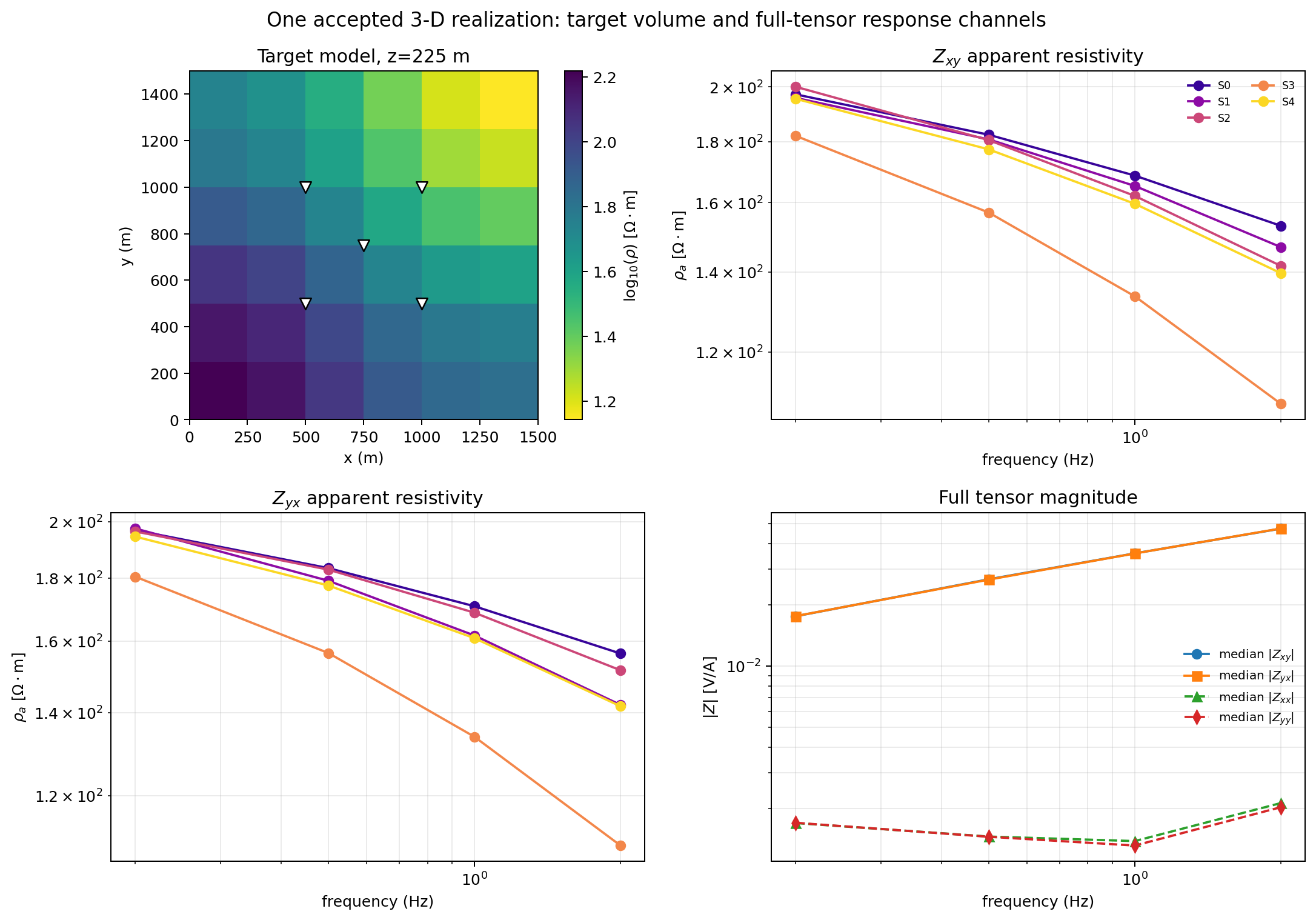
One 3-D target volume slice beside apparent-resistivity curves for Zxy and Zyx at five stations, and full-tensor impedance magnitude including the diagonal components. — One accepted, moderately heterogeneous realization. Upper-left: the target volume’s shallowest slice, with five receivers (white triangles). Upper-right and lower-left: \(Z_{xy}\) and \(Z_{yx}\) apparent resistivity per station, colour-matched between panels. Lower-right: median impedance magnitude across all five stations for all four tensor components.#

The lower-right panel is where the contrast with the half-space check above lands. \(|Z_{xy}|\) and \(|Z_{yx}|\) are close enough here to overlap almost completely, which is itself informative – this particular realization’s correlated field is heterogeneous but not strongly anisotropic in its overall response. \(|Z_{xx}|\) and \(|Z_{yy}|\) sit roughly an order of magnitude lower, clearly separated from zero rather than pinned at machine precision the way the half-space check’s diagonal was. That gap is the genuine 3-D distortion signal this module exists to expose to training: a station near the resistive body in the upper-left panel sees a different response than a station near the boundary at the lower-right, in a way two independent 2-D cross-sections through the same volume would not reproduce identically.

6.3.8.6. Handing this to noise, agents, or training#

This module deliberately stops at a clean, forward-consistent response, the same boundary 2-D Maxwell training-data generation draws. Realistic field-like corruption – heteroscedastic noise, dropout, static shift, and distortion fitted from a real survey’s own quality control – is Domain-gap and noise simulation’s job, kept separate so a clean control volume always exists independently of whatever noise model sits on top of it later.

Inv3DAgent’s physics="mt3d" mode (AI inversion agents) is the nearest consumer: it builds a Maxwell3DDatasetConfig from the survey’s own real station geometry, calls generate_3d_maxwell_dataset() internally, and reports a genuine held-out recovery check ((9)) against known synthetic truth rather than fabricating one. Its mesh_safety_factor, max_mesh_cells, cells_per_skin_depth, geology_grid_nx_ny, and geology_grid_nz constructor parameters map directly onto this module’s own configuration fields, so a mesh-guard message raised through the agent is diagnosed with exactly the tools this page already covers.

Beyond a single agent, a Maxwell3DDataset’s train/ validation/test partitions and its DatasetManifest are the same shape of input Loss functions for scientific inversion trains against and Recovery, residual, and OOD diagnostics reports evidence from – the realization-level split guards against the same leakage Canonical data contracts enforces for any other split. A training corpus should still make its partition sizes explicit before committing a solve budget this much larger per realization than 2-D Maxwell training-data generation’s:

>>> plan_grid = GeologyGrid.regular_3d(
...     nx=8, ny=8, nz=8, dx_m=200.0, dy_m=200.0, dz_m=100.0
... )
>>> station_xy = [
...     [x, y] for x in (400.0, 800.0, 1200.0) for y in (400.0, 800.0, 1200.0)
... ]
>>> production_plan = Maxwell3DDatasetConfig(
...     dataset_id="volume-3d-v2",
...     grid=plan_grid,
...     correlation_length_x_m=(400.0, 1000.0),
...     correlation_length_y_m=(400.0, 1000.0),
...     correlation_length_z_m=(150.0, 400.0),
...     frequencies_hz=[20.0, 5.0, 1.0],
...     station_xy_m=station_xy,
...     n_realizations=200,
...     seed=42,
...     cells_per_skin_depth=8.0,
...     max_mesh_cells=20_000,
...     validation_fraction=0.15,
...     test_fraction=0.15,
... )
>>> production_plan.n_realizations
200
>>> production_plan.validation_fraction, production_plan.test_fraction
(0.15, 0.15)
>>> production_plan.grid.shape
(8, 8, 8)
>>> production_plan.station_xy_m.shape
(9, 2)

Two hundred realizations at up to 20,000 solver cells each is a configuration to budget compute for deliberately, not a default to reach for. As with 2-D Maxwell training-data generation’s closing example, this is a shape check, not an adequacy claim: whether 200 realizations, this correlation range, and this frequency band are sufficient depends on the geological diversity and precision a specific downstream evaluation needs, and that judgement belongs with Recovery, residual, and OOD diagnostics, not with this configuration object. After generation, read partition sizes from dataset.split.sizes rather than back-computing them from the requested fractions, since rejected solves are removed before the split is applied, and persist dataset.manifest alongside every realization’s clean realization_id so a later noise variant from Domain-gap and noise simulation never crosses a partition boundary.