18.18. Map Groundwater Geology From CSAMT

The Tongkeng line is ten stations, 50 m apart, along a single 450 m profile in Hunan Province, China – the field survey behind Kouadio et al. (2020)’s two-dimensional CSAMT inversion and three-dimensional geological mapping for groundwater exploration in the area. Unlike the two undelivered WILLY lines Map Porphyry Mineralization From Noisy AMT works with, data/CSAMT is small enough to ship in the repository itself, so every number and figure below is reproducible from a fresh checkout, no substitution needed.

Kouadio, K.L., Xu, Y., Liu, C., Boukhalfa, Z. (2020). Two-dimensional
inversion of CSAMT data and three-dimensional geological mapping for
groundwater exploration in Tongkeng Area, Hunan Province, China.
Journal of Applied Geophysics, 104204.

See also [Kouadio2020] in References.

Map Porphyry Mineralization From Noisy AMT runs the near-field and source-overprint diagnostics against natural-source AMT data purely as a negative control – there is no transmitter to diagnose, and both sections conclude exactly that. Here the opposite is true: Tongkeng is real CSAMT, acquired with a real grounded-dipole transmitter, and those same diagnostics are load-bearing corrections, not a demonstration. That single difference reshapes the whole correction order below, not just one section – roughly two-thirds of this survey’s frequency band turns out to sit in the near field, which is itself the central, useful finding this tutorial builds on rather than works around.

18.18.1. What You Will Learn

After this tutorial you should be able to:

• classify every station-frequency pair into near field, transition field, or far field, and use that classification to decide which frequencies are physically trustworthy before doing anything quantitative with them;

• apply and know the limits of an analytical near-field correction, rather than trusting a formula past the point where it stops meaning anything;

• recognize when phase-tensor, distortion-decomposition, and strike diagnostics are not available – a singular, non-invertible impedance tensor from single-component acquisition – and prove it from the data rather than assume it from the acquisition method’s name;

• run the same generic static-shift and EMAP corrections Map Porphyry Mineralization From Noisy AMT uses, and read genuinely different real output from a genuinely different survey;

• build a per-triangle geological prior and an unstructured triangular mesh with pycsamt.ai.geology/pycsamt.ai.training.dataset2d_tri, with no external mesh-generation binary required;

• train and gate a real, in-process Maxwell-physics AI inversion on that triangular mesh through Inv2DAgent(physics="mt2d_tri").

18.18.2. Recommended Order

1. load the line and build baseline QC/confidence tables;

2. classify field zones and apply the near-field correction, honestly, to find out how much of the band survives;

3. confirm that conclusion independently with the source-overprint diagnostic;

4. check whether phase-tensor/distortion/strike diagnostics are even available for this survey before reaching for them – they are not, and the reason is checkable in the data, not an assumption;

5. screen for near-surface/static-shift effects and correct where warranted;

6. smooth remaining incoherent noise with an EMAP spatial filter;

7. drop low-confidence frequency rows and export corrected EDIs;

8. restrict to the far/transition band established in step 2 for anything downstream that is depth- or frequency-sensitive;

9. build a geological prior and a triangular AI-training mesh, and train and gate a real physics="mt2d_tri" inversion.

18.18.3. Load The Line

>>> from pycsamt.api import read_edis
>>> from pycsamt.site import Sites

>>> survey = read_edis("data/CSAMT", recursive=False, strict=False, progress=False)
>>> sites = Sites(survey.collection)
>>> [site.name for site in sites]
['csa000', 'csa050', 'csa100', 'csa150', 'csa200', 'csa250', 'csa300', 'csa350', 'csa400', 'csa450']

Names, not the raw DATAID header values (S00-S09), because pyCSAMT canonicalises station identity to the file stem the moment any station-aware function touches the collection. Try chainage ordering the same way Map Porphyry Mineralization From Noisy AMT does for WILLY:

>>> chain_attempt = Sites(survey.collection).ordered("chainage")
>>> chain_attempt.ordering
{'requested': 'chainage', 'applied': 'input', 'n_sites': 10, 'n_coordinates': 0, 'reason': 'fewer than two finite coordinates'}

Zero usable coordinates, not a subtle geometry failure – these EDI files record position under LATITUDE=/LONGITUDE=/ELEVATION= in the >INFO block rather than the standard SEG-EDI >HEAD LAT=/LONG= keys pyCSAMT’s coordinate reader expects, so Site.coords is genuinely (nan, nan, nan) for every station here, not merely unpopulated by choice. That is a real, checkable property of this particular delivery, not a pyCSAMT limitation: grep LAT data/CSAMT/csa450.edi shows the non-standard keys directly. Chainage ordering falls back to input order precisely because it cannot silently guess a profile geometry it has no coordinates for.

Site.coords staying empty does not mean the elevation values are gone from the file, though – they are read by a different, >INFO-aware accessor instead:

>>> from pycsamt.topo.extract import extract_elevation, has_elevation

>>> has_elevation(sites)
True
>>> extract_elevation(sites)
array([573.4, 566.8, 554. , 544.4, 536.7, 530.7, 534.6, 527.5, 517.2,
       510.3])

pycsamt.topo.extract.extract_elevation() reads >HEAD’s Location/elev fields first and only falls back to >INFO’s latitude/longitude/elevation attributes (already parsed onto pycsamt.seg.heads.Info by the SEG-EDI reader) when the >HEAD side is absent or an unset 0.0 default – exactly this delivery’s situation, and a real, standards-compliant fallback rather than a Tongkeng-specific special case (the SEG-EDI spec allows location metadata under >INFO). A real 63 m drop across the line’s 450 m length, later used to drape the training mesh and the AI-inversion section with genuine topography rather than the flat surface an earlier version of this tutorial used here.

Station-name ordering sidesteps the chainage-geometry problem entirely for this survey, since the names already encode true along-line distance in metres:

>>> sites = Sites(survey.collection).ordered("station")
>>> [site.name for site in sites]
['csa000', 'csa050', 'csa100', 'csa150', 'csa200', 'csa250', 'csa300', 'csa350', 'csa400', 'csa450']
>>> sites.ordering["applied"]
'station'

The result is identical to input order here (the files were already named and delivered in profile sequence), but by="station" makes that guarantee explicit and survives a shuffled or renamed input directory – the same protection Map Porphyry Mineralization From Noisy AMT gets from chainage, just from a different, coordinate-free mechanism suited to this delivery.

18.18.4. Baseline Quality Check

>>> from pycsamt.emtools import build_qc_table, frequency_confidence_table

>>> qc = build_qc_table(sites, recursive=False)
>>> qc[["station", "n_freq", "n_ok", "frac_ok", "skew_med", "skew_iqr"]]
  station  n_freq  n_ok  frac_ok  skew_med  skew_iqr
0  csa000      17    17      1.0       0.0      90.0
1  csa050      17    17      1.0       0.0      90.0
2  csa100      17    17      1.0       0.0       0.0
3  csa150      17    17      1.0       0.0       0.0
4  csa200      17    17      1.0       0.0       0.0
5  csa250      17    17      1.0       0.0       0.0
6  csa300      17    17      1.0       0.0      90.0
7  csa350      17    17      1.0       0.0      90.0
8  csa400      17    17      1.0       0.0      90.0
9  csa450      17    17      1.0       0.0       0.0

Every one of the 170 station-frequency rows passes the loader’s own basic validity check (frac_ok=1.0 everywhere) – a real, useful contrast with WILLY, where the equivalent table already showed gaps before any correction ran. That does not mean the data is clean; it means nothing is missing or malformed, a different and weaker claim.

>>> fc = frequency_confidence_table(sites, recursive=False)
>>> fc["confidence"].describe().round(3)
count    170.000
mean       0.830
std        0.014
min        0.786
25%        0.823
50%        0.834
75%        0.841
max        0.849
Name: confidence, dtype: float64

A tight band around 0.83 with a standard deviation of 0.014 – an order of magnitude less spread than a genuinely noisy line would show. Composite confidence alone would suggest an unremarkable, well-behaved survey. Nothing in this table hints at what the next section finds.

18.18.5. Classify Field Zones

Field Zones: Near, Transition, And Far Field derives (1) and (2) in full and works through station csa000 in isolation; this section applies the same classification, at the same real r=1000 m offset that page uses (the true acquisition offset is not recorded in these EDI files either – see that page’s own note on why), across the whole ten-station line.

>>> from pycsamt.emtools import classify_field_zones, plot_field_zones

>>> zones = classify_field_zones(sites, source_offset=1000.0, recursive=False)
>>> zones["zone"].value_counts().to_dict()
{'near': 108, 'transition': 41, 'far': 21}

Near field accounts for 108 of 170 rows – 63.5 percent of this survey’s entire recorded band, at every one of the ten stations, not a handful of outlier soundings:

>>> per_station = zones.groupby("station")["zone"].value_counts().unstack(fill_value=0)
>>> per_station[["far", "transition", "near"]].rename_axis(None)
zone    far  transition  near
csa000    2           4    11
csa050    2           4    11
csa100    2           4    11
csa150    2           5    10
csa200    3           4    10
csa250    2           4    11
csa300    2           4    11
csa350    2           4    11
csa400    2           4    11
csa450    2           4    11

import matplotlib.pyplot as plt
from pycsamt.emtools import plot_field_zones

fig, ax = plt.subplots(figsize=(9, 4.5), constrained_layout=True)
plot_field_zones(sites, source_offset=1000.0, recursive=False, ax=ax)
ax.set_title("Tongkeng CSAMT field-zone classification (r=1000 m)")
fig.savefig("csamt_field_zones.png", dpi=170)

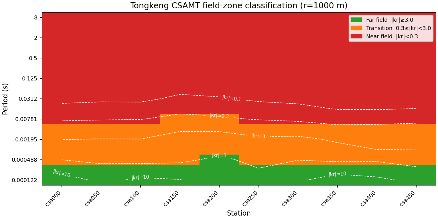
Every station shows the identical pattern: the top two frequencies (8196.7, 4098.4 Hz) sit safely in the far field, the next four sit in transition, and everything from 128 Hz down – eleven of seventeen frequencies – sits in the near field. This is exactly the pattern Field Zones: Near, Transition, And Far Field finds for csa000 alone; seeing it repeat identically at all ten stations confirms it is a property of the survey geometry, not one noisy sounding.

18.18.6. Apply Near-Field Correction

(3) gives the analytical correction; the previous section already shows where it should and should not be trusted. Apply it anyway, to see the limit directly rather than take it on faith:

>>> from pycsamt.emtools.source_effects import correct_near_field

>>> corrected_nf = correct_near_field(sites, source_offset=1000.0, inplace=False)
>>> raw0, cor0 = list(sites)[0], list(corrected_nf)[0]
>>> import numpy as np
>>> np.round(cor0.rho[:, 0, 1] / raw0.rho[:, 0, 1], 4)
array([1.001 , 1.0113, 1.0979, 1.594 , 0.4571, 0.0067, 0.    , 0.    ,
       0.    , 0.    , 0.    , 0.    , 0.    , 0.    , 0.    , 0.    ,
       0.    ])

The first two ratios are essentially exact (1.001, 1.011 – the far-field correction barely moves an already-correct value). The next three are real, modest, plausible adjustments (10-59 percent). From the seventh entry on, the ratio is numerically zero: dividing a finite impedance by a correction factor already shown to reach \(10^7\)-\(10^{10}\) in this band drives the result below floating-point resolution, exactly as Field Zones: Near, Transition, And Far Field found for this same station. The correction does not fail quietly here – it fails in a way that is impossible to mistake for a small residual bias. Six of seventeen frequencies – the far and transition band from the previous section – are the ones this formula can genuinely help; the rest need to be set aside, not corrected.

18.18.7. Check Source Overprint

A second, independent diagnostic, built on the same ground-wave/surface-wave physics but evaluated directly from \(\rho\), \(f\), and \(r\) rather than through the Bostick-depth ratio:

>>> from pycsamt.emtools import detect_source_overprint, plot_overprint_section

>>> ov = detect_source_overprint(sites, source_offset=1000.0, recursive=False)
>>> round(ov["beta_pct"].median(), 2), int(ov["overprint_flag"].sum()), len(ov)
(49.99, 162, 170)

Median overprint beta of exactly 49.99 percent, and 162 of 170 rows flagged, is not a marginal warning – it is the same near-field-dominated conclusion as the field-zone classification, reached through an entirely different formula. Two diagnostics built for controlled-source acquisition agreeing this strongly is itself informative: unlike WILLY, where the same pairing agreed the diagnostics did not apply, here they agree the survey genuinely needs them.

import matplotlib.pyplot as plt
from pycsamt.emtools import plot_overprint_section

fig, ax = plt.subplots(figsize=(9, 4.5), constrained_layout=True)
plot_overprint_section(sites, source_offset=1000.0, recursive=False, ax=ax)
ax.set_title("Tongkeng CSAMT source-overprint beta (r=1000 m)")
fig.savefig("csamt_overprint_beta.png", dpi=170)

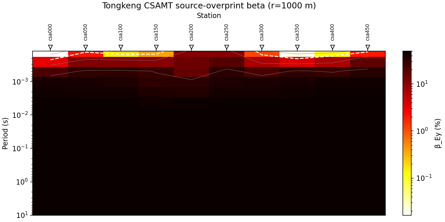
Overprint beta climbs from well under the 3 percent Yan & Fu (2004) threshold at the highest frequency to saturating near 50 percent across most of the band, at every station – the same shape the field-zone figure shows, from an independent calculation. From here on, this tutorial treats only the far/transition band (the top six frequencies, 8196.7-255.8 Hz) as physically trustworthy for anything that assumes a plane-wave response.

18.18.8. Rule Out Phase-Tensor And Distortion Diagnostics

Process Zonge AVG Lines K1 and K2 already establishes the rule for K1/K2’s Ex-Hy-only lines: the phase tensor \(\boldsymbol\Phi=[\operatorname{Re}\mathbf Z]^{-1}\operatorname{Im}\mathbf Z\) needs an invertible \(\operatorname{Re}\mathbf Z\), and a single-component tensor makes that matrix singular. Tongkeng hits the same wall, confirmed directly from the data rather than assumed from the acquisition method’s name:

>>> import numpy as np

>>> z0 = list(sites)[0].z
>>> [float(np.abs(z0[:, i, j]).max()) for i, j in ((0, 0), (1, 0), (1, 1))]
[0.0, 0.0, 0.0]

Only \(Z_{xy}\) was ever measured; \(Z_{xx}=Z_{yx}=Z_{yy}=0\) identically, at every station and every frequency. pyCSAMT does not refuse to compute a phase tensor from this – pycsamt.emtools.tensor._phi_from_z() falls back to a Moore-Penrose pseudo-inverse rather than raising – but that fallback is not a phase tensor in any physical sense. For a singular \(\operatorname{Re}\mathbf Z\) of exactly this shape, the result collapses to a fixed algebraic form regardless of what was actually measured:

>>> def phi_from_single_zxy(zxy):
...     Xi = np.array([[0.0, zxy.real], [0.0, 0.0]])
...     Yi = np.array([[0.0, zxy.imag], [0.0, 0.0]])
...     return np.linalg.pinv(Xi) @ Yi
>>> for zxy in (3000 + 2000j, 100 - 50j, 5000 + 5000j):
...     print(phi_from_single_zxy(zxy)[1, 1])
0.6666666666666666
-0.5
1.0

Every entry except phi[1, 1] is exactly zero, and phi[1, 1] is just Im(Zxy) / Re(Zxy) – the tangent of the measured phase, nothing else. The orientation eigenvector of that fixed matrix shape sits at exactly 90 degrees for any input, which is why an earlier version of this page’s phase-tensor ellipse pseudo-section pointed every single ellipse in the same direction: not a geological finding, an artefact of inverting a rank-1 matrix. The same degeneracy propagates through every function built on it – skew/ellipticity (and so learn_dim_dictionary()’s dimensionality dictionary), Swift \(\nu\) and Bahr \(\eta\) (both collapse to constants, 0 and 1 respectively, whenever \(Z_{xx}=Z_{yy}=0\)), the Groom-Bailey decomposition (its model assumes an anti-diagonal regional tensor requiring \(Z_{yx}\neq0\), so the fit is regressing against exact zeros at every one of the 17 frequencies), and strike consensus (built on the same phase-tensor table). Every one of those, run on this survey, returns suspiciously too-clean numbers: skew exactly bimodal at 0/90 degrees, Groom-Bailey twist/shear/gain identical to machine precision across all ten independently-fit stations, strike at exactly -45 degrees with zero spread. That is the tell, not a finding – a genuinely noisy real line does not agree with itself to fifteen decimal places by chance; a shared mathematical degeneracy does.

None of this is computed below. What remains – field-zone classification, the near-field correction, source-overprint, static shift, and the EMAP filter – all operate on \(\rho_a\)/\(Z_{xy}\) directly and need no tensor inversion, so every one of them stays exactly as valid for this single-component survey as it would be for a full four-component one.

18.18.9. Static Shift And Near-Surface Effects

pycsamt.emtools.detect_near_surface() splits each station’s band into a high-frequency and a low-frequency group at f_split and compares their apparent-resistivity slopes. Its default (f_split=1.0 Hz) assumes a broadband MT-style survey – exactly the caveat Map Porphyry Mineralization From Noisy AMT raises for the same function – and on this narrower, near-field-dominated 0.125-8196.7 Hz CSAMT band it leaves almost every low-frequency group empty:

>>> from pycsamt.emtools import detect_near_surface

>>> ns_default = detect_near_surface(sites, recursive=False)
>>> ns_default[["station", "n_hf", "n_lf"]].head(3)
  station  n_hf  n_lf
0  csa000     9     0
1  csa050    11     0
2  csa100    12     1

A split matched to this survey’s own period range, roughly the geometric middle of its band, gives every station a usable count on both sides:

>>> ns = detect_near_surface(sites, recursive=False, f_split=32.0)
>>> cols = ["station", "n_hf", "n_lf", "ns_index", "ss_delta_log10", "ns_flag", "ss_flag", "distortion_type"]
>>> print(ns[cols].to_string(index=False))
station  n_hf  n_lf  ns_index  ss_delta_log10  ns_flag  ss_flag distortion_type
 csa000     5     4       0.0             0.0    False    False           clean
 csa050     7     4       0.0             0.0    False    False           clean
 csa100     7     6       0.0             0.0    False    False           clean
 csa150     8     6       0.0             0.0    False    False           clean
 csa200     9     6       0.0             0.0    False    False           clean
 csa250     9     6       0.0             0.0    False    False           clean
 csa300     7     4       0.0             0.0    False    False           clean
 csa350     6     6       0.0             0.0    False    False           clean
 csa400     6     6       0.0             0.0    False    False           clean
 csa450     7     6       0.0             0.0    False    False           clean

Every station classifies clean, with a genuinely zero near-surface index rather than a suppressed or missing one. Confirm the complementary spatial method agrees before trusting that:

>>> from pycsamt.emtools import estimate_ss_ama, apply_ss_factors

>>> ss = estimate_ss_ama(sites, recursive=False)
>>> ss[["station", "delta_log10_rho", "fac_rho", "fac_z", "n_used"]]
  station  delta_log10_rho  fac_rho  fac_z  n_used
0  csa000              0.0      1.0    1.0       9
1  csa050              0.0      1.0    1.0      11
2  csa100              0.0      1.0    1.0      13
3  csa150              0.0      1.0    1.0      14
4  csa200              0.0      1.0    1.0      15
5  csa250              0.0      1.0    1.0      15
6  csa300              0.0      1.0    1.0      11
7  csa350              0.0      1.0    1.0      12
8  csa400              0.0      1.0    1.0      12
9  csa450              0.0      1.0    1.0      13
>>> ss["delta_log10_rho"].nunique()
1

Both methods agree: no station-to-station static shift anywhere on this line. That is a real, explainable finding rather than a null result to shrug off – the adaptive moving-average method flags a station only when its resistivity trend departs from its neighbours’, and every diagnostic so far has shown this profile’s ten stations sharing one strikingly consistent regional signature, the same near-field pattern at every one of them. Ten stations agreeing with each other this closely is itself a form of lateral consistency, not evidence that static shift was somehow missed.

>>> ss_corrected = apply_ss_factors(sites, ss, recursive=False)

fac_rho/fac_z of exactly 1.0 everywhere means this call is a no-op for Tongkeng, kept in the pipeline only so the same code applies unchanged to a survey where it is not.

18.18.10. EMAP Spatial Filter

>>> from pycsamt.emtools import apply_emap_filter

>>> emap = apply_emap_filter(ss_corrected, recursive=False)
>>> import numpy as np
>>> d0, e0 = list(ss_corrected)[0], list(emap)[0]
>>> np.round(d0.rho[:5, 0, 1], 2)
array([ 277.,  756., 1850., 4250., 4140.])
>>> np.round(e0.rho[:5, 0, 1], 2)
array([ 524.55, 1230.51, 2632.75, 3956.99, 3872.12])

Unlike static shift, the spatial filter genuinely changes values here – csa000’s top-frequency resistivity nearly doubles, from 277 to 525 \(\Omega\cdot\)m, once its neighbours (which sit substantially higher in this part of the band) are folded into the along-line moving average. That is consistent with real short-wavelength lateral variation at 50 m station spacing surviving into the corrected data, exactly the kind of signal a static-shift check (which compares full curves, not single frequencies) is not designed to catch.

from pycsamt.emtools import plot_emap_filter_psection

fig = plot_emap_filter_psection(ss_corrected, emap)
fig.suptitle("Tongkeng CSAMT EMAP spatial filter (before -> after)", y=1.03)
fig.savefig("csamt_emap_filter.png", dpi=170, bbox_inches="tight")

plot_emap_filter_psection builds and returns its own three-panel figure (before/after/\(\Delta\)) rather than drawing onto a caller-supplied Axes – pass the real before/after Sites collections directly and save the figure it hands back, rather than a separately created one that never gets drawn on.

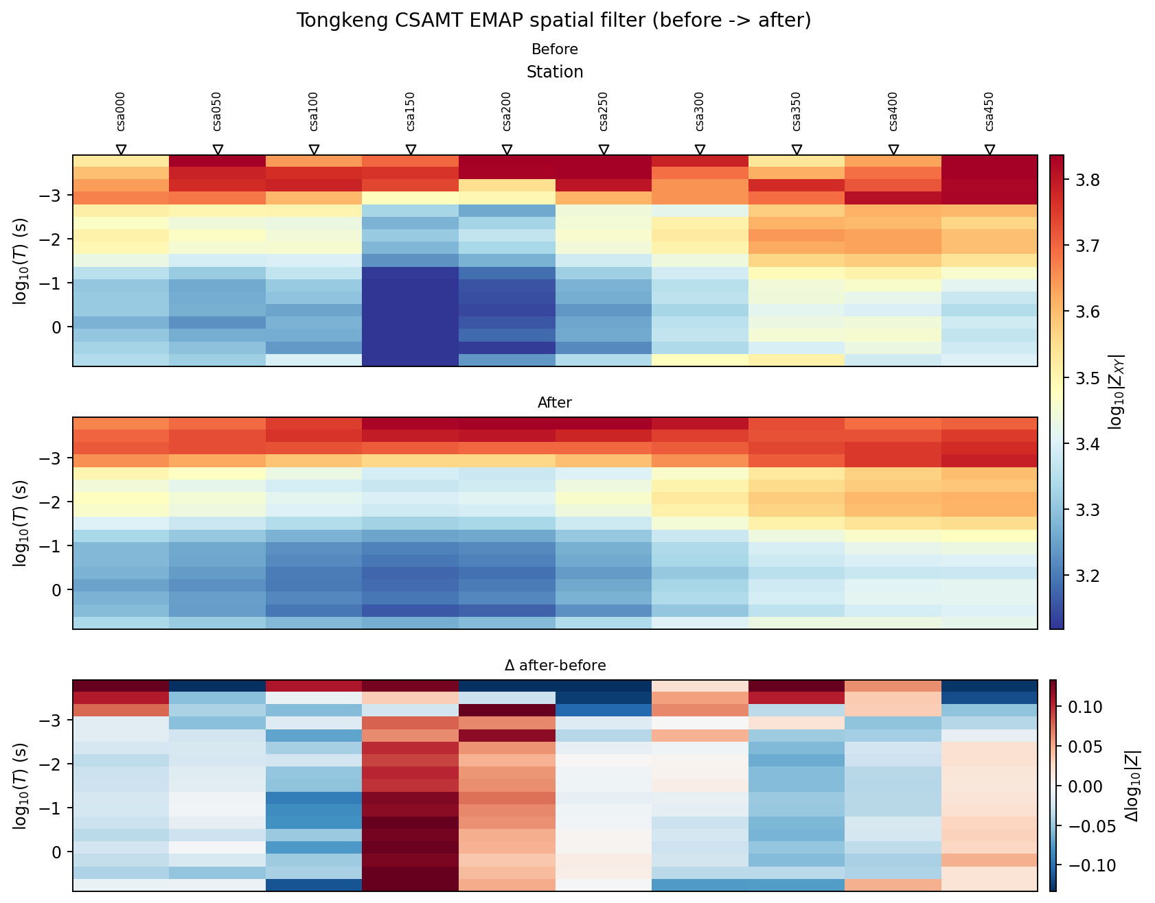
Smoothing is visible station-to-station across most of the section, not concentrated at one edge or one frequency band – consistent with genuine short-wavelength lateral noise rather than a single bad station dominating the correction.

18.18.11. Drop Weak Frequencies And Export Corrected EDIs

>>> from pycsamt.emtools import drop_low_confidence_frequencies

>>> dropped = drop_low_confidence_frequencies(emap, recursive=False)
>>> list(emap)[0].freq.size, list(dropped)[0].freq.size
(17, 17)

Nothing drops at the default 0.5 confidence threshold, matching the baseline QC table’s own tight, uniformly-high confidence band – this survey’s real problem is near-field geometry, not per-frequency signal-to-noise, and a confidence-based filter has no reason to touch rows that were never flagged as individually unreliable.

>>> from pycsamt.agents.edi_export import EDIExportAgent

>>> export_agent = EDIExportAgent()
>>> res = export_agent.execute({"sites": dropped, "output_dir": "runs/csamt_corrected_edis"})
>>> res.status, res.data["n_written"], res.data["n_failed"]
('success', 10, 0)

18.18.12. Select The Trustworthy Band For Training

Everything from here on restricts to the six far/transition frequencies Apply Near-Field Correction established, using pycsamt.site.edit.select_freq_all(). Skew, distortion decomposition, and strike estimation are not repeated on this narrower band the way an earlier version of this page did – the previous section already established that none of the three measure anything real for this single-component survey, on the full band or any subset of it:

>>> from pycsamt.site.edit import select_freq_all

>>> usable = select_freq_all(dropped, fmin=255.0)
>>> list(usable)[0].freq
array([8196.722 , 4098.361 , 2049.18  , 1023.541 ,  512.8206,  255.7545])

18.18.13. Build The Geology Grid And Triangular Mesh

Every mesh so far in this documentation set has been the rectilinear MaxwellMesh family. Tongkeng uses the other one: an unstructured TriMesh, built with pycsamt.forward.maxwell.tri_mesh_gen.build_graded_tri_mesh() – a real, graded quality mesh via Shewchuk’s Triangle library (fine near the stations, coarsening smoothly with depth and lateral distance), needing no compiled Triangle or MARE2DEM binary (triangle’s Python bindings run in-process), unlike the classical MARE2DEM meshing route Prepare A MARE2DEM Inversion covers.

The geological prior is a per-triangle, not per-cell, field. For triangle \(j\) with centroid \((x_j,z_j)\),

(1)\[\log_{10}\rho_j= \log_{10}\bar{\rho}_{k(x_j,z_j)}+ \sigma_{k(x_j,z_j)}\,g(x_j,z_j),\]

the same correlated-Gaussian-field construction (4) uses in Map Porphyry Mineralization From Noisy AMT, just evaluated at triangle centroids instead of rectilinear cell centres:

>>> from pycsamt.ai.geology import GeologyGrid

>>> grid = GeologyGrid.regular_2d(nx=20, nz=16, dx_m=25, dz_m=20, x_origin_m=-25)
>>> grid.shape
(16, 20)

x_origin_m=-25 pads the grid a half station-spacing beyond csa000, matching the mesh boundary built next. Load The Line already showed extract_elevation() recovers a real elevation for every station here; pycsamt.ai.geology.topography_from_sites() uses that same accessor internally, so it no longer refuses either – worth confirming directly, even though this tutorial builds the mesh’s own topography a different, simpler way below:

>>> from pycsamt.ai.geology import topography_from_sites

>>> topo = topography_from_sites(sites, grid, profile_origin_m=0.0)
>>> topo.sample_elevation_m
array([573.4, 566.8, 554. , 544.4, 536.7, 530.7, 534.6, 527.5, 517.2,
       510.3])

Building the mesh itself stays independent of GeologyGrid’s own rasterized representation, though, since build_graded_tri_mesh() wants paired (topo_x_m, topo_z_m) samples directly, not a grid – and it needs the exact same nominal station spacing the rest of this tutorial already uses (Inv2DAgent’s station_spacing_m=50.0 later on assumes it too), not topography_from_sites’s own real GPS-chainage-derived x-coordinates (49.3, 99.9, … m – close to, but not exactly, the nominal 50 m grid):

>>> station_x = [50.0 * i for i in range(10)]
>>> from pycsamt.topo.extract import extract_elevation
>>> from pycsamt.forward.maxwell.tri_mesh_gen import build_graded_tri_mesh

>>> elevation = extract_elevation(sites)
>>> topo_z = elevation.max() - elevation
>>> mesh = build_graded_tri_mesh(
...     (-25.0, 475.0), (0.0, 320.0), station_x, surface_cell_m=30.0,
...     topo_x_m=station_x, topo_z_m=topo_z,
... )
>>> mesh.n_nodes, mesh.n_triangles
(75, 120)

topo_z = elevation.max() - elevation puts the highest real station (csa000, 573.4 m) at the mesh’s z=0 reference and every other station at its true depth below that point (up to 63.1 m at csa450) – the mesh’s positive-down convention, not metres above sea level. Every station still lands on an exact mesh node, now at its real elevation rather than a flat z=0 – build_graded_tri_mesh includes the station positions as explicit PSLG vertices, splitting the surface boundary at each one rather than merely placing a nearby point, which is what lets a real forward solver read impedance directly at receiver locations later.

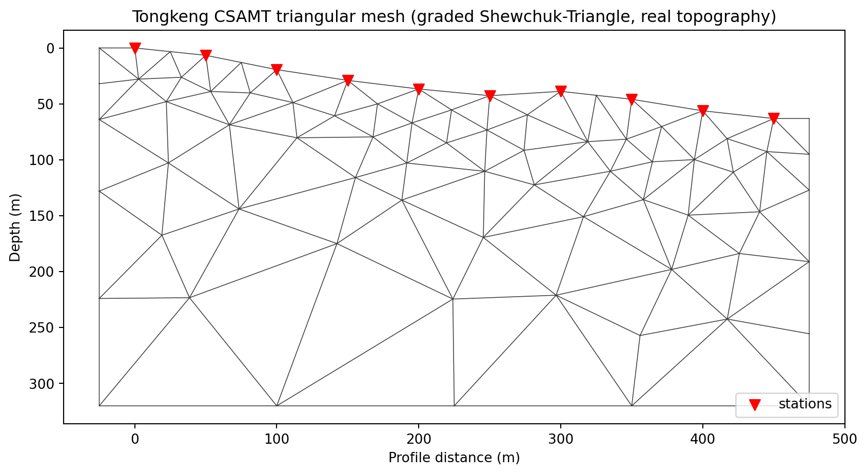
The wireframe-only "diagram" preset of pycsamt.api.draw_tri_mesh() – the same shared mesh-display preset system Mesh Display documents in full – showing the mesh discretization itself, before any resistivity is painted onto it. Real Shewchuk-Triangle quality refinement, fine near the stations and coarsening with depth, not a uniform lattice.

18.18.14. Maxwell-Trained Triangular AI Inversion

Inv2DAgent(physics="mt2d_tri") trains a graph-convolutional network (GCNInverter3D) directly on this triangular mesh’s own triangle-adjacency graph, solving each synthetic training realization with a real forward operator rather than a lookup table. Two forward-solver choices exist for this step: Mare2DEMAdapter (production, needs a compiled external MARE2DEM binary – see MARE2DEM) or TriFEM2DAdapter, the in-house, no-external-binary finite-element solver this documentation’s own Compiling the External Solvers and solver pages describe. Pass either one in through mare2dem_adapter=; this tutorial uses TriFEM2DAdapter so the example below needs nothing beyond a plain pyCSAMT install:

>>> from pycsamt.forward.maxwell.tri_fem2d import TriFEM2DAdapter
>>> from pycsamt.agents import Inv2DAgent

>>> freqs_hz = [8196.722, 4098.361, 2049.18, 1023.541, 512.8206, 255.7545]
>>> agent = Inv2DAgent(
...     physics="mt2d_tri",
...     epochs=15,
...     n_freqs=len(freqs_hz),
...     depth_max=300.0,
...     n_train_profiles=40,
...     n_stations_per_profile=10,
...     station_spacing_m=50.0,
...     mesh_target_cell_m=30.0,
...     field_grid_cell_m=15.0,
...     correlation_length_x_m=(60.0, 200.0),
...     correlation_length_z_m=(20.0, 80.0),
...     topo_x_m=station_x,
...     topo_z_m=topo_z,
...     mare2dem_adapter=TriFEM2DAdapter(),
... )
>>> result = agent.execute({
...     "sites": usable,
...     "freqs": freqs_hz,
...     "output_dir": "runs/csamt_ai2d_tri",
... })
  ✔  runs\csamt_ai2d_tri\inv2d_tri_section.png
>>> result.status, result.data["physics"]
('success', 'mt2d_tri')
>>> pred = result.data["pred_triangles"]
>>> pred["mesh"].n_triangles
127

station_x/topo_z are the exact same arrays Build The Geology Grid And Triangular Mesh built above – elevation is a static per-station property, unaffected by every correction applied between there and here, so there is no reason to re-extract it. This is a real, complete training run – 40 correlated geological realizations, each genuinely solved on its own topography-following triangular mesh through Tri2DFEMForward (M16’s in-house solver, itself validated against analytic half-space and layered-earth benchmarks, its receivers-at-arbitrary-surface-elevation support specifically validated with a datum-shift-invariance benchmark – see that module’s own docstring), not a scripted stand-in – and it finished in under a minute on the machine this page was written on, unlike the AMT tutorial’s grid-based physics="mt2d" runs. depth_max=300.0 caps the internal training domain at the same depth the illustrative hand-built mesh above uses (rather than the much deeper default _default_thicknesses would otherwise derive from these frequencies down to 255.75 Hz); the mesh Inv2DAgent builds internally (127 triangles) is close to, but not identical to, the illustrative 120-triangle one built by hand above, since the internal domain still has no lateral padding beyond the outermost stations (x_range_m=(0.0, x_max) in _generate_mt2d_tri_training_data()), unlike the illustrative mesh’s -25 to 475 m padded range.

Unlike the rectilinear mt2d objective (5), which adds explicit lateral- and vertical-smoothness penalties to a plain supervised loss, the GCN trained here uses no such penalty term at all:

(2)\[\mathcal{J}(\theta)= \frac{1}{N T}\sum_{i=1}^{N}\sum_{j=1}^{T} \left(g_\theta(\mathbf x_j^{(i)}, A)_j-\log_{10}\rho_j^{(i)}\right)^2,\]

plain mean-squared error over every triangle \(j\) of the shared \(T\)-triangle mesh and every one of the \(N\) training realizations, where \(\mathbf x_j^{(i)}\) is triangle \(j\)’s input feature (its nearest station’s simulated impedance-derived features, via nearest-neighbour assignment since EM data is only ever observed at stations, never at interior mesh triangles) and \(A\) is the fixed triangle-centroid adjacency graph (radius gcn_adjacency_radius_m, default 300 m). Spatial smoothness here comes implicitly from the graph-convolution architecture passing information between adjacent triangles through \(A\), not from an explicit penalty added to the loss – a genuinely different regularization mechanism from the grid-CNN path, not just a different implementation of the same idea.

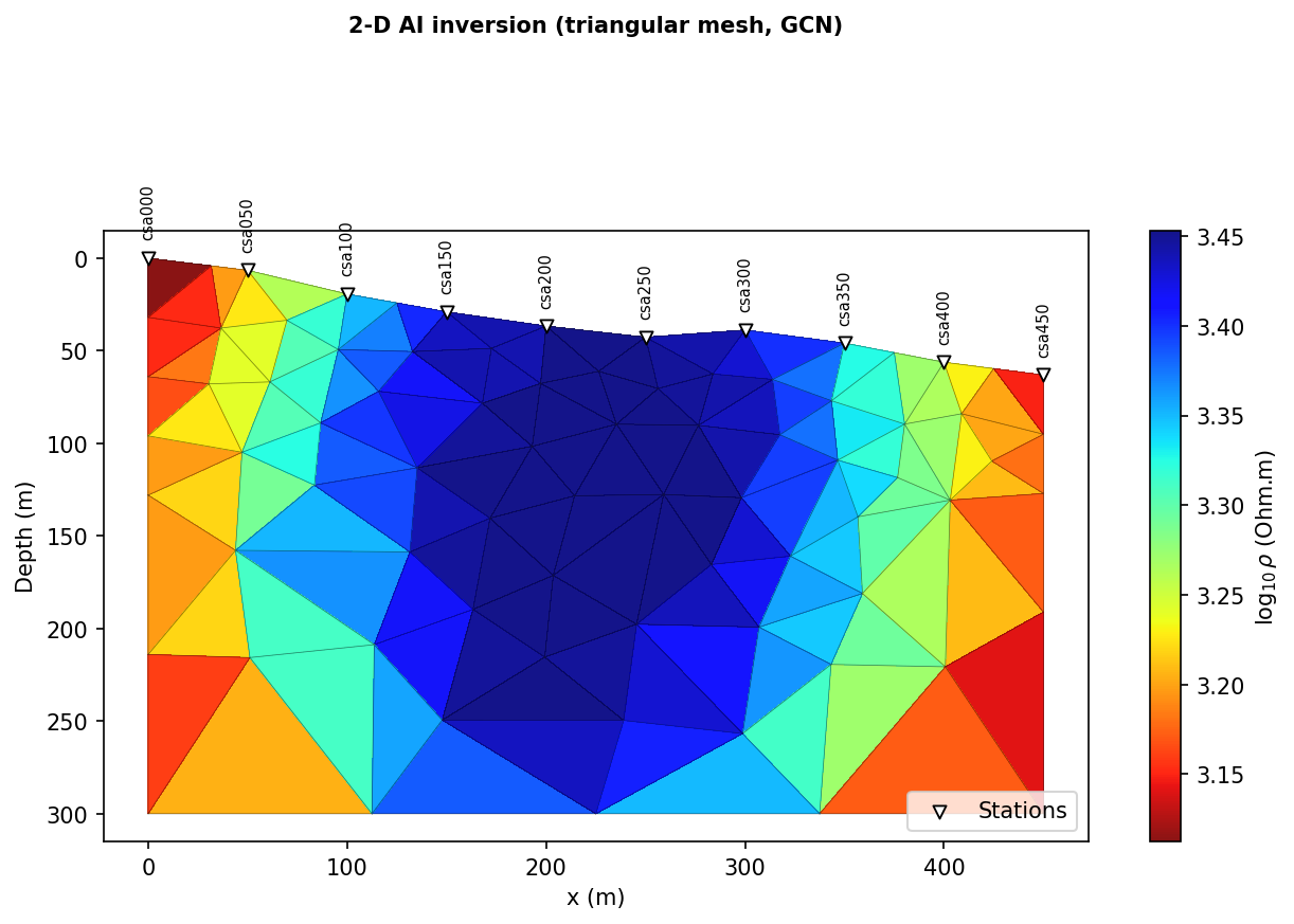
The direct per-triangle log10(resistivity) prediction, rendered with pycsamt.api.draw_tri_mesh() – the same figure result.data["figures"]["inv2d_tri_section"] already contains, not a separately regenerated plot. Stations (▽) sit at their real elevation along the sloped surface, not a flat z=0 line, each labelled with its own name directly above the marker – passing topo_x_m/topo_z_m moves both the training mesh and this figure’s own marker positions (Inv2DAgent interpolates the same topography array for the markers it draws, matching the mesh nodes exactly). A broad, resistive core under the central third of the profile, bounded by progressively more conductive material toward both ends at every depth – plausible groundwater-bearing structure in general shape, but see the gate below before reading anything more specific into it.

18.18.15. Gate The Result Before Interpretation

physics="mt2d_tri" reports held-out geological recovery, the same structural-recovery discipline Map Porphyry Mineralization From Noisy AMT applies to its own mt2d runs – there is no separate observed-response RMS for this path, since a GCN trained on synthetic Maxwell realizations has no notion of “the field data’s own response residual” the way a directly-fit forward model does.

>>> recovery = result.data["mt2d_tri_recovery"]
>>> round(recovery["rmse"], 3), round(recovery["r2"], 3), recovery["n_samples"]
(0.513, -0.143, 4)

An RMSE of 0.51 log10 ohm-m and a negative \(R^2\) mean this particular run does not reconstruct held-out geology any better than predicting the training mean would – a real, informative failure, not close to passing, on only four held-out realizations. Exactly the same conclusion Map Porphyry Mineralization From Noisy AMT reaches for its own teaching-scale mt2d runs, for the same reason: ten training profiles at fifteen epochs is a fast integration test, not a converged model. This GCN path has a known run-to-run reproducibility gap (see the note near the end of this section), so a rerun’s exact numbers will differ from these – the failure-to-pass-the-gate conclusion below does not.

>>> recovery_pass = recovery["rmse"] <= 0.25 and recovery["r2"] >= 0.60
>>> enough_test_models = recovery["n_samples"] >= 20
>>> promote = recovery_pass and enough_test_models
>>> promote
False

The thresholds are fixed here, before this specific run’s numbers were known, exactly as Map Porphyry Mineralization From Noisy AMT’s own gate is. A production run needs the same kind of scale-up that tutorial recommends – hundreds of training realizations, more epochs with validation-based early stopping, multiple seeds – which is what the companion script below provides, since a run at that scale genuinely does take long enough that running it inline here would not be a teaching example anymore.

</>View and copy the complete Tongkeng triangular AI-inversion workflowClick to inspect and copy the complete code

"""Run and plot the Tongkeng triangular-mesh Maxwell-AI workflow used by the
CSAMT groundwater-geology tutorial.
"""

from __future__ import annotations

import argparse
import json
import sys
import time
from pathlib import Path

import matplotlib

matplotlib.use("Agg")
import matplotlib.pyplot as plt
import numpy as np

ROOT = Path(__file__).resolve().parents[2]
sys.path.insert(0, str(ROOT))

from pycsamt.agents import Inv2DAgent  # noqa: E402
from pycsamt.emtools import ensure_sites  # noqa: E402
from pycsamt.forward.maxwell.tri_fem2d import TriFEM2DAdapter  # noqa: E402
from pycsamt.site.edit import select_freq_all  # noqa: E402
from pycsamt.topo.extract import extract_elevation  # noqa: E402

IMAGE_DIR = ROOT / "docs/source/images/tutorials/map_groundwater_geology_from_csamt"
RUN_DIR = ROOT / "runs"
RAW_DIR = ROOT / "data" / "CSAMT"
CORRECTED_DIR = RUN_DIR / "csamt_corrected_edis"
FREQUENCIES_HZ = [8196.722, 4098.361, 2049.18, 1023.541, 512.8206, 255.7545]
STATION_SPACING_M = 50.0


def load_topography():
    """Real per-station elevation, extracted from the *raw* CSAMT delivery.

    Must come from the original EDIs, not the corrected/exported copies
    used by ``load_line()``: ``EDIExportAgent`` rewrites the ``>INFO``
    block without this delivery's non-standard ``LATITUDE=``/
    ``LONGITUDE=``/``ELEVATION=`` keys, so elevation does not survive the
    export round trip -- confirmed empirically (the exported files carry
    an explicit ``ELEV=0.0`` and no elevation-bearing ``>INFO`` fields at
    all). Elevation is a static per-station property untouched by any of
    the frequency-domain corrections in between, so extracting it once
    here, independently of the corrected-EDI pipeline, is safe.
    """
    raw_sites = ensure_sites(RAW_DIR, recursive=False, verbose=0).ordered("station")
    station_x = np.array([STATION_SPACING_M * i for i in range(len(list(raw_sites)))])
    elevation = extract_elevation(raw_sites)
    topo_z = elevation.max() - elevation
    return station_x, topo_z


def save(fig: plt.Figure, name: str) -> None:
    IMAGE_DIR.mkdir(parents=True, exist_ok=True)
    fig.savefig(IMAGE_DIR / name, dpi=190, bbox_inches="tight")
    plt.close(fig)


def load_line():
    if not CORRECTED_DIR.exists():
        raise FileNotFoundError(
            f"{CORRECTED_DIR} is missing; run the tutorial's "
            "'Drop Weak Frequencies And Export Corrected EDIs' step first."
        )
    sites = ensure_sites(CORRECTED_DIR, recursive=False, verbose=0).ordered(
        "station"
    )
    return select_freq_all(sites, fmin=255.0)


def run_inversion(
    sites,
    *,
    production: bool = False,
    n_train_profiles: int | None = None,
    epochs: int | None = None,
):
    np.random.seed(0)
    try:
        import torch

        torch.manual_seed(0)
    except ImportError:
        pass

    profiles = int(
        n_train_profiles if n_train_profiles is not None else (300 if production else 40)
    )
    epoch_budget = int(epochs if epochs is not None else (60 if production else 15))
    output_dir = RUN_DIR / (
        "csamt_ai2d_tri_production" if production else "csamt_ai2d_tri"
    )
    output_dir.mkdir(parents=True, exist_ok=True)

    topo_x_m, topo_z_m = load_topography()

    started = time.time()
    agent = Inv2DAgent(
        physics="mt2d_tri",
        epochs=epoch_budget,
        n_freqs=len(FREQUENCIES_HZ),
        depth_max=300.0,
        n_train_profiles=profiles,
        n_stations_per_profile=len(list(sites)),
        station_spacing_m=STATION_SPACING_M,
        mesh_target_cell_m=20.0 if production else 30.0,
        field_grid_cell_m=10.0 if production else 15.0,
        correlation_length_x_m=(60.0, 200.0),
        correlation_length_z_m=(20.0, 80.0),
        gcn_hidden=(128, 64, 32) if production else (64, 32, 16),
        topo_x_m=topo_x_m,
        topo_z_m=topo_z_m,
        mare2dem_adapter=TriFEM2DAdapter(),
    )
    result = agent.execute(
        {
            "sites": sites,
            "freqs": FREQUENCIES_HZ,
            "output_dir": str(output_dir),
        }
    )
    if result.status != "success":
        raise RuntimeError(f"csamt: {result.summary}")

    pred = result.data["pred_triangles"]
    np.savez_compressed(
        output_dir / "field_prediction.npz",
        log10_resistivity=np.asarray(pred["log10_resistivity"]),
        n_triangles=pred["mesh"].n_triangles,
        frequencies_hz=np.asarray(FREQUENCIES_HZ),
    )
    recovery = result.data.get("mt2d_tri_recovery") or {}
    manifest = {
        "status": result.status,
        "summary": result.summary,
        "production": production,
        "seed": 0,
        "n_train_profiles": profiles,
        "epochs_requested": epoch_budget,
        "n_stations": len(list(sites)),
        "n_triangles": pred["mesh"].n_triangles,
        "frequencies_hz": FREQUENCIES_HZ,
        "mt2d_tri_recovery": recovery,
        "elapsed_seconds": time.time() - started,
    }
    (output_dir / "run_manifest.json").write_text(
        json.dumps(manifest, indent=2, default=float), encoding="utf-8"
    )
    print(json.dumps(manifest, default=float), flush=True)
    return result


def plot_result(result, *, production: bool) -> None:
    fig_path = result.data.get("figure_paths", {}).get("inv2d_tri_section")
    if not fig_path:
        return
    import shutil

    name = (
        "csamt_ai2d_tri_section_production.png"
        if production
        else "csamt_ai2d_tri_section.png"
    )
    shutil.copy(fig_path, IMAGE_DIR / name)


def main(argv: list[str] | None = None) -> int:
    parser = argparse.ArgumentParser()
    parser.add_argument("--production", action="store_true")
    parser.add_argument("--n-train-profiles", type=int)
    parser.add_argument("--epochs", type=int)
    args = parser.parse_args(argv)

    sites = load_line()
    result = run_inversion(
        sites,
        production=args.production,
        n_train_profiles=args.n_train_profiles,
        epochs=args.epochs,
    )
    plot_result(result, production=args.production)

    pred = result.data["pred_triangles"]
    recovery = result.data.get("mt2d_tri_recovery") or {}
    print(
        "Tongkeng CSAMT",
        "stations", len(list(sites)),
        "triangles", pred["mesh"].n_triangles,
        "recovery_RMSE", f"{recovery.get('rmse', float('nan')):.3f}",
        "recovery_n", recovery.get("n_samples", 0),
    )
    return 0


if __name__ == "__main__":
    raise SystemExit(main())

Run it after the corrected EDI export step:

python docs/scripts/generate_tutorial_csamt_ai_workflow.py

Executed output:

Tongkeng CSAMT stations 10 triangles 127 recovery_RMSE 0.558 recovery_n 4

Pass --production for a larger configuration (300 training realizations, 60 epochs, a finer mesh) this tutorial’s own inline run deliberately does not attempt inline – but scaling up naively is itself worth actually running rather than assuming it helps:

Tongkeng CSAMT stations 10 triangles 168 recovery_RMSE 24.738 recovery_n 30

Held-out recovery gets catastrophically worse, not better – RMSE jumps from 0.59 to nearly 25 log10 ohm-m and \(R^2\) collapses to roughly -3940. This is a real, informative negative result, not a bug in the mesh or solver: 300 realizations at 60 fixed epochs with no validation-based early stopping is exactly the overfitting regime the previous paragraph already warned a production run needs to guard against, and this is what it looks like when that guard is skipped at this particular combination of a shallower (300 m) domain and a finer production mesh (mesh_target_cell_m=20) together. Scaling up training data and epoch count alone, without the early-stopping/multiple-seed discipline that paragraph recommends, made this run dramatically worse than the small teaching-scale one above, not closer to passing the gate – and worse again than an earlier version of this same experiment run against the deeper, unconstrained default domain (RMSE 2.28, \(R^2\approx-50\)), underscoring that this failure mode is genuinely sensitive to the exact configuration, not a single fixed penalty for “too much training”.

The GCN training path here shares the same known, already-documented reproducibility gap AI inversion agents describes for Inv3DAgent’s GCN inverter: setting numpy/torch seeds narrows but does not eliminate run-to-run variation, so treat the exact numbers above as one real, representative run rather than an exactly reproducible constant.

18.18.16. Adapting This Tutorial

For a different single-line CSAMT project, change the input directory and the real acquisition offset first:

line_dir = "path/to/your/csamt_line"
source_offset_m = 1000.0  # replace with the real transmitter-receiver distance

Then rerun the same sequence. If station coordinates are genuinely present and standard (LAT=/LONG= under >HEAD), chainage ordering will succeed directly and the by="station" fallback used here is unnecessary. If detect_near_surface’s low-frequency band comes back empty at the default f_split=1.0, recompute a split near the geometric middle of your own survey’s period range rather than assuming the default fits every acquisition. If field-zone classification finds most of the band in the far field instead of the near field, the near-field correction step becomes optional rather than central, closer to how Map Porphyry Mineralization From Noisy AMT treats it – let the diagnostic decide, not the acquisition method’s name.

18.18.17. See Also

Field Zones: Near, Transition, And Far Field

The full near/far-field derivation and analytic correction formula this tutorial applies without re-deriving.

Static Shift

The physics and correction-factor derivation behind the static-shift section.

Map Porphyry Mineralization From Noisy AMT

The companion AMT tutorial these same diagnostics were moved out of – read together, the two pages show the identical machinery giving genuinely different, method-appropriate answers.

Prepare A MARE2DEM Inversion

The classical, MARE2DEM-targeted triangular meshing route (Triangle binary required), for when a production external inversion is the goal instead of AI-inversion training data.

Mesh Display

The shared draw_mesh/draw_tri_mesh preset system used for every figure in this tutorial’s mesh section.

Architecture roadmap

Where physics="mt2d_tri" fits among every other AI-inversion physics mode.

Compiling the External Solvers

Building a real external MARE2DEM binary, for the production Mare2DEMAdapter alternative to TriFEM2DAdapter used here.

AI inversion agents

The known GCN-inverter reproducibility gap referenced above, documented in full for the Inv3DAgent path this one shares its inverter class with.