11.27.5. Profile-Level Anomaly Detection#

Machine-Learning Quality Scoring and Quality-Control Confidence Scoring both score data quality at the (station, frequency) grain – one number per cell. That grain is right for deciding whether to mask a single bad frequency, but it cannot flag a station whose entire spectrum is unusual in shape or level even though every individual frequency looks locally reasonable. AnomalyDetector works at the opposite grain: one feature vector per station, built by flattening prepare_z_features()’s (n_components, n_freqs) array, and one anomaly score per station.

The detector is a fully connected autoencoder – the same reconstruction-error idea as Learned Spectral Denoising, but on whole flattened station vectors instead of per-channel sequences, and used as a diagnostic score rather than to produce a cleaned output:

(1)#\[\hat{\mathbf{x}} = g(f(\mathbf{x})), \qquad s_i = \frac{\|\mathbf{x}_i - \hat{\mathbf{x}}_i\|_2^2}{d}\]

where \(f : \mathbb{R}^d \to \mathbb{R}^k\) is the encoder (\(k \ll d\), set by latent_dim) and \(g\) the decoder. A station is flagged when its reconstruction error \(s_i\) exceeds the threshold_percentile-th percentile (default the 95th) of the training scores – so, by construction, roughly 5% of a representative training set is expected to be flagged. When neither PyTorch nor TensorFlow is installed, the same interface falls back to PCA reconstruction via sklearn.decomposition.PCA.

11.27.5.1. Fitting and scoring#

>>> from pycsamt.ai.processing import AnomalyDetector, prepare_z_features
>>> X = prepare_z_features(sites, n_components=4)
>>> n_sites, n_comp, n_freq = X.shape
>>> X_flat = X.reshape(n_sites, n_comp * n_freq)
>>> X_flat.shape
(28, 212)
>>> det = AnomalyDetector(latent_dim=8, channels=(32, 16))
>>> det.fit(X_flat, epochs=150, seed=0, verbose=False)
AnomalyDetector(n_features=212, latent_dim=8, torch, fitted)
>>> det.threshold_
2.4401
>>> flags = det.flag_anomalies(X_flat)
>>> int(flags.sum())
2

With latent_dim=8 and 212 raw features, the bottleneck compresses each station to 4% of its original size – tight enough that a station whose spectrum shape genuinely differs from the rest of the line cannot be reconstructed as well as a typical one.

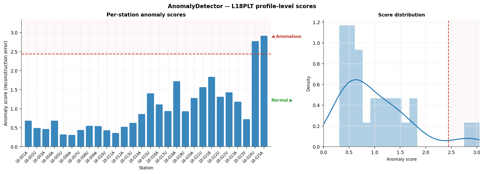
plot_anomaly_summary() – per-station scores (a) and their pooled distribution (b), with the fitted threshold shared between both panels.#

Two stations cross the threshold, both by a wide margin over the rest of the line: 18-024U and 18-025A – the last two, adjacent stations on the profile. 18-024U is one of the seven stations whose Machine-Learning Quality Scoring score collapsed under the hard Swift-skew rule – a station already flagged as electrically unusual by a completely different method agreeing with the anomaly detector here. Both flagged stations also share a trait neither the rule-based QC score nor a single-channel view would surface directly: their \(\phi_{xy}\) curves are noticeably noisier than the rest of the line (standard deviation \(\approx 28^\circ\) and \(25^\circ\), against a \(15^\circ\) median across all 28 stations) – a station-wide, cross-channel pattern rather than a handful of bad frequencies, exactly the kind of anomaly a whole-spectrum reconstruction-error model is built to catch and a per-frequency QC rule, which only ever looks at one station at a time against a fixed threshold, has no mechanism to compare against its neighbours to find.

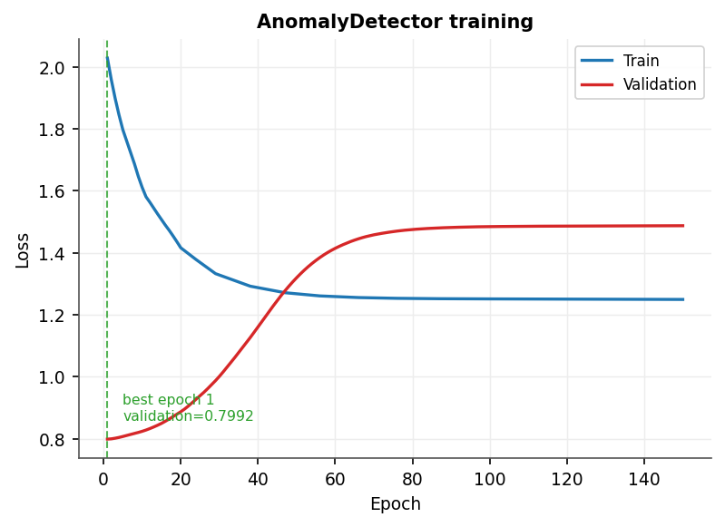
plot_training_history() on the fitted detector.#

Warning

With only 28 training stations (about 25 after the validation split), this training curve is a textbook small-sample case: training loss keeps falling while validation loss bottoms out early (here, around epoch 7) and drifts back up afterward as the network starts memorizing individual training stations rather than the shared structure across them. fit() already restores the lowest-validation-loss weights automatically, so the deployed model is unaffected – but the curve itself is a reminder that a profile this short gives the Isolation Forest fallback and this network comparably little to generalize from. Prefer more stations, a smaller latent_dim, or the threshold_percentile rule-of-thumb over a literal reading of the loss curve when the training set is this small.

11.27.5.2. Sites in, filtered sites out#

apply() closes the same sites-in / sites-out loop as Learned Spectral Denoising’s apply() and Machine-Learning Quality Scoring’s apply(), but its shape is different: rather than mutating Z.z in place, it drops flagged stations outright via Sites.select(), since the detector scores whole stations, not station-frequency cells. There is therefore no inplace option here – Sites.select() always returns a new container, and so does this method.

>>> clean_sites = det.apply(sites, n_components=4)
>>> len(list(sites)), len(list(clean_sites))
(28, 26)
>>> {s.name for s in sites} - {s.name for s in clean_sites}
{'18-024U', '18-025A'}

n_components (and freq_ref/log_amp when set explicitly) must reproduce the exact feature layout the detector was fitted on – apply() checks the flattened length against the fitted n_features and raises ValueError rather than silently scoring a mismatched vector when they disagree.

Note

The two dropped stations above match the ones read off the summary figure earlier on this page – reran here through a different code path for illustration, not a different result. Because the network’s weight initialization is not seeded (see the warning in Learned Spectral Denoising about fit(seed=...) covering only the data split and synthetic noise, not PyTorch’s own initialization RNG), an independent re-fit of the detector can occasionally flag a different pair of borderline stations even with the same data and threshold_percentile.

11.27.5.3. Parameters#

latent_dim (default 32) is the main capacity knob: too large and the network can reconstruct almost anything, including real anomalies, driving every score toward zero; too small and it cannot represent normal variability either, inflating scores across the board. channels sets the encoder hidden widths (decoder mirrors them). threshold_percentile (default 95.0) trades false positives against false negatives directly – lower it to flag more stations for review, raise it to flag only the most extreme outliers.

Full signatures: AnomalyDetector, plot_anomaly_scores(), plot_anomaly_score_distribution(), and plot_anomaly_summary().

Point load_l18() at your own EDI folder to adapt this script